A Tour of Where Process Data Is Born

📍 Where we are: Having followed one data point through its lifecycle in The Lifecycle of a Data Point, we now zoom out to the whole factory — and re-walk the entire monoclonal-antibody process as a chain of places where process data is born.

In the previous chapter we traced a single measurement from the instant a sensor or analyst created it, through capture, contextualization, and archival — the data lifecycle that is the spine of everything in this book. We also learned that raw data without metadata (the context that says what, when, where, and under which conditions a value was recorded) is just noise. Now comes the natural next question: where do all those data points actually come from? To answer it, we take a walking tour of a biopharmaceutical plant — but with a twist. Instead of asking "what does each machine make?", we ask "what data does each machine emit?"

The simple version

Imagine touring a busy restaurant kitchen, but you can only see the order tickets, not the food. Each station — the grill, the fryer, the plating bench — spits out its own kind of ticket at its own rhythm. The bioprocess is the same. Every piece of equipment is quietly printing a different kind of "ticket," and our job is to read the factory as a stream of tickets rather than a stream of liquid.

What this chapter covers

We will reframe the standard process map as a data map, station by station — upstream cell culture, downstream purification, fill-finish, and quality control. Along the way we introduce four ideas the rest of the book builds on: that each station emits a characteristic data shape; the difference between measuring during the process and afterward; how soft sensors fuse the two; and batch genealogy, the chaining of every station's data into one coherent story. We close by looking at how continuous manufacturing changes the very shape of the data.

The process map is a data map

A monoclonal antibody (mAb) is a therapeutic protein grown by living cells — the kind of medicine used to treat cancers and autoimmune disease. Making one is a relay race of unit operations: discrete processing steps, each performed by dedicated equipment (a bioreactor, a chromatography column, a filter). The traditional way to draw this process is as a flow of material — cells in, purified drug out.

But there is a second, parallel flow that never appears on the material diagram: data. A foundational principle of modern bioprocessing, formalized by regulators in the FDA's Process Analytical Technology (PAT) framework — guidance that encourages building quality into a process by measuring it as it runs rather than only testing the final product [8] — is that quality should be understood and controlled through measurement at each step [1]. Every unit operation, in other words, is also a data station. It generates a characteristic signature of sensor readings, probe traces, and analyzer outputs that, taken together, describe what happened inside [2].

Adopt that lens and the plant looks different. Here is the same mAb process, drawn as the data each station emits.

Each station emits a different kind of data; the manufacturing line is also a data-generating line. Original diagram by the authors, created with AI assistance.

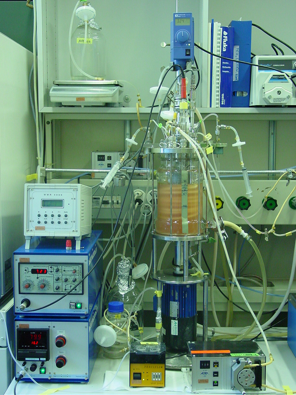A bench-scale bioreactor instrumented with probes — an upstream data source generating continuous temperature, pH, and dissolved-oxygen traces. This is a bench/development-scale vessel, shown because it carries the same instrumentation as the much larger production tank described below. Bench-scale bioreactor. Image by Jonas Schenk, public domain, via Wikimedia Commons.

Upstream: the bioreactor as a time-series fountain

Upstream means cell culture and product generation — everything from growing the cells through harvest, the point at which the culture is ready to be separated from the cells. (Harvest, and the clarification step right after it, is the conventional boundary between upstream and downstream.) Upstream's centerpiece is the bioreactor — the large, instrumented tank where the cells live and secrete product, physically described in the manufacturing book's chapter on the production bioreactor. As a data station, the bioreactor is the noisiest and most continuous one in the whole plant.

Why each station's data has a shape: scalar, spectral, event

Probes inside the tank read temperature, pH (acidity), and dissolved oxygen (the oxygen available for the cells to breathe) every few seconds, producing dense time-series data — a stream of values stamped with the time they were taken. A typical sample might land in a historian as a row like BR101.Temp.PV,2026-06-13T08:00:00Z,37.5,degC — one tag, one timestamp, one value, one unit. The bioreactor does not carry just those three tags, though: a production vessel reports temperature, pH, DO, agitation, several gas flows, head pressure, level or weight, plus their setpoints and a handful of derived tags — a dozen-plus channels — so across the full tag set several hundred rows land every minute. Layered on top are discrete events: each nutrient feed, each dose of base to correct pH, each sample drawn.

And increasingly, spectroscopic probes such as Raman — which shine light into the broth and infer its chemistry from how that light scatters — turn the bioreactor into a multivariate data source in its own right: a single in-line Raman probe has been shown to track glucose, lactate, glutamine, and viable cell density (the culture's two key nutrients, its main waste product, and the count of living cells) simultaneously and in real time [4], so what used to be four separate lab pulls (samples sent to the lab) becomes one continuous stream. Each Raman scan is a full spectrum of intensity versus wavenumber — several hundred points — and the four analyte concentrations are not read off directly but predicted from it by a multivariate calibration (PLS) model, the same kind of model that can drift as the culture ages. The next chapter gives Raman and its cousins their proper introduction; here it is enough to see that the bioreactor alone can emit dozens of correlated channels at once.

The deeper point is that the bioreactor already mixes three shapes of data — a dense scalar time-series (temperature), a high-dimensional spectral vector (the Raman scan), and timestamped events (a feed). No single station emits just one shape, and no single store fits all three. Recognizing the shape of each signal is the first design decision a data architecture makes, because shape dictates everything downstream: how it is stored, how it is compressed, and how it can be queried. We make this concrete in the one-record-many-shapes section below.

In-line, on-line, at-line, off-line: four locations and their latencies

This introduces our first big distinction: not all measurements are taken in the same place relative to the process stream. A measurement is in-line when the sensor sits inside the process stream and reads it in place, with no sample removed — the temperature probe immersed in the broth is in-line, and a result arrives continuously. When a technician instead pulls a sample to read it nearby, soon after, the measurement is at-line. And there is a third location, on-line, that sits between in-line and at-line — a small side-stream is automatically diverted out of the process, measured, and often returned — which is why "online" data is not quite the same as "in-line" data. These three — in-line, on-line, and at-line — are the process-analyzer modes the FDA's PAT framework defines [8]. Set against them is off-line measurement (a sample taken away and analyzed later in a separate lab), the conventional approach PAT aims to reduce by moving measurement closer to the process. The next chapter, on instruments and sensors, splits all four locations apart in detail. For now, hold one idea: the bioreactor mixes a flood of continuous in-line (and some on-line) data with a trickle of at-line and off-line lab results that must later be reunited.

The four locations are not just a vocabulary; they describe a single, hard trade-off. As you move left to right — in-line to off-line — latency rises and frequency falls, but definitiveness climbs: an in-line probe gives you a fast indirect proxy, while an off-line HPLC (high-performance liquid chromatography) gives you the slow reference-grade number that actually releases the batch (the formal decision to approve it for use).

The four measurement locations trade latency and frequency for definitiveness; PAT moves measurement leftward toward the process. Original diagram by the authors, created with AI assistance.

Time-series density and reconciliation: fusing continuous and sparse

Reuniting the flood and the trickle is itself a data problem, and it is where soft sensors earn their keep. A soft sensor is a model that fuses frequent online signals with sparse at-line or off-line values to estimate a process variable that no single probe measures directly — biomass, growth rate, or glucose uptake, inferred in real time for monitoring and control rather than measured outright [6]. For instance, a soft sensor might infer real-time biomass concentration from frequent Raman spectral readings paired with the occasional manual cell count, letting the control system adjust feeding before an analyst's next lab result arrives hours later. The online stream gives the soft sensor its rhythm; the occasional lab value keeps it honest. This is more than a convenience: it is why soft sensors sit at the heart of the data architecture, because they are how a plant turns a fast-but-indirect signal and a slow-but-trustworthy one into a single number a controller can act on.

The reconciliation runs deeper than two clocks ticking at different rates. The in-line stream and the lab pull rarely line up in time — the manual cell count is drawn at 08:00 but does not return until 11:00, by which point the bioreactor has emitted ten thousand more readings — so fusing them means aligning a value to a process instant it was never stamped with, and deciding which signal to trust when they disagree. That alignment-and-trust problem is the live edge of upstream data management, and it is the heart of the open challenge we close this chapter with.

Downstream: clarification, traces, and phase events

Downstream is purification — separating the antibody from everything else the cells produced. It opens with clarification and capture: the harvested broth is run through a centrifuge and depth filters to remove cells and debris before the first column. Even this housekeeping step is a data station — it emits turbidity (a measure of how cloudy the stream still is), filter pressure, and flow readings, and a rising pressure here signals a filter loading up just as it does anywhere else.

Downstream's workhorse, though, is chromatography, in which the protein mixture is pumped through a column packed with resin that grabs some molecules and lets others flow past — the physical step covered in the manufacturing book's chapter on capture chromatography. The first such step for an antibody is Protein A capture — affinity resin that grips the antibody by its Fc stem while host-cell proteins and DNA wash past — and it is worth grounding the data in its real unit operation, because the numbers a station emits only mean something against the operation that made them. The skids that run it — process-scale systems such as Cytiva's ÄKTA process line or Sartorius's Resolute — are not just pumps and valves; as a data station, a chromatography skid is a chorus of continuous traces plus sharp phase events. Detectors at the column outlet continuously record UV absorbance at 280 nm (a proxy for how much protein is passing — it might sit near zero during loading and spike past 2.5 absorbance units at the peak of elution), conductivity (a proxy for salt concentration), and pH [5]. Overlaid are the named phases — load, wash, elute, regenerate (load the mixture onto the resin, wash impurities away, elute the captured product off, then regenerate/clean the column for reuse) — each a timestamped event marking a deliberate change in conditions.

Two derived numbers ride on those raw traces and are themselves data the genealogy must carry. The first is the breakthrough shoulder: load past the resin's dynamic binding capacity (DBC) — the grams of antibody a litre of resin holds at the running flow rate, typically 40 to 80 g/L — and unbound product begins escaping out the bottom, visible as a quiet rise in the load-phase UV trace. The second is the leached Protein A trend: a little of the grabber ligand sheds off the beads each cycle, so a per-batch parts-per-million result climbs as the resin ages toward its validated cycle-life limit. Neither is read from one instant; both are computed across the trace and across the resin's reuse history, which is why a chromatography record is incomplete unless it is bound to the column lot and its cycle count, not just the timestamp. The decisive moment is when to start and stop collecting the purified product, the pooling decision: the operator collects only the slice of the elution peak between two cut points, judged against a UV threshold in column volumes. That cut-point choice is a real-time quality decision — set too late and the aggregate-rich tail drags into the pool — so it must be recorded as a reviewable, attributable part of the batch record, exactly the chromatography data-integrity expectation PIC/S PI 041 frames. Conventionally the pooling call is judged from the standard UV trace; more advanced approaches measure it directly — in one large-scale demonstration, an on-line HPLC analyzer made the real-time pooling call from the data itself [5], though that remains a demonstrated technique rather than routine practice. When the third book builds an open-source downstream-chromatography module, this same chorus of traces plus phase events — and the derived breakthrough, pooling, and leached-ligand decisions — is exactly the data it has to capture and timestamp.

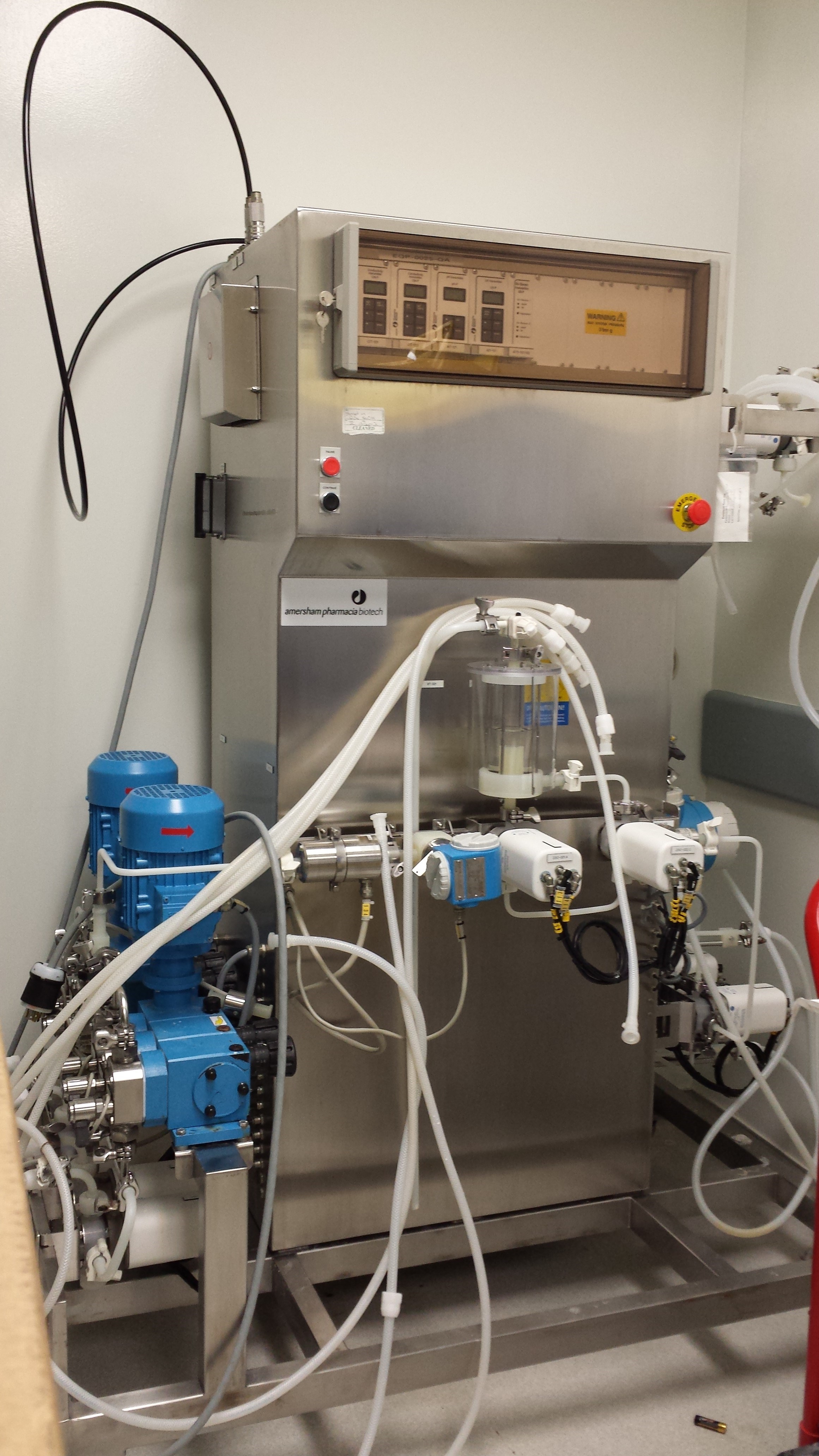A process chromatography skid. Each purification step emits UV, conductivity, and pH traces plus discrete phase-transition events. (The unit shown is an earlier Amersham Pharmacia Biotech system; the ÄKTA and Resolute lines are named only as current examples.) Image by Kitmondo Lab, CC BY 2.0 (https://creativecommons.org/licenses/by/2.0/), via Wikimedia Commons (File: Amersham Pharmacia Biotech chromotography skid.jpg).

Sandwiched between chromatography steps is tangential flow filtration (TFF) — pushing liquid across a membrane to concentrate the product or swap its buffer. Its data signature is simpler but just as telling: flux (how fast liquid crosses the membrane) and transmembrane pressure (the pressure difference driving it across). A creeping pressure rise is the membrane's way of reporting that it is fouling.

note

Notice the pattern. Each station has a shape of data. The bioreactor's is a long dense time-series; chromatography's is a bundle of traces punctuated by events; TFF's is a pair of pressure-and-flow signals. Recognizing these shapes is half the battle of managing the data, because each shape wants to be stored and analyzed differently. These station signatures are the raw material of the four families of data from Chapter 1 — the bioreactor and chromatography traces feed the process-data family, the QC chromatograms the quality family — all bound to the same batch identity (written s88.batch because it is keyed to the ISA-88 batch model, introduced below).

Fill-finish and QC: the last drops and the final word

Fill-finish is where bulk drug becomes the vials or syringes a patient receives. Its data is a blend: a fill-weight for every container (a continuous stream of scalar measurements), machine-vision images checking each unit for defects, and environmental monitoring — particle counts and microbial samples proving the room stayed clean.

Finally comes quality control (QC) — the analytical lab that confirms the batch is what it claims to be, the step the manufacturing book describes under QC and release. QC is the archetype of offline data. Instruments such as HPLC produce chromatograms (curves) and tables of results hours or days after the sample was drawn, using methods validated to the standard set out in ICH Q2(R2) — a guideline from the International Council for Harmonisation (ICH), the body that harmonises pharmaceutical-quality requirements across the major regulators; this one is the 2023 revision of the guideline for validating analytical procedures, paired with the new ICH Q14 on analytical-procedure development [9]. These are direct analytical measurements, and they carry the regulator-grade weight that releases the batch — which is exactly why they must be linked back, unambiguously, to the batch and the station they describe.

One record format, many shapes

Every station above emits the same atomic unit — a single tagged reading — and the whole edifice of batch genealogy, reconciliation, and regulatory trust rests on getting that one record right. The previous chapter, the lifecycle of a data point, already dissects this record field by field, on the bioreactor's dissolved-oxygen value 2026-01-05T00:00:00Z, BR101.DO.PV, 40.8224, %sat, 192, BATCH-2026-001 — six fields (tag, timestamp, value, unit, quality, batch_id), each a deliberate choice that turns a bare number into a small identity card. We do not repeat that dissection here.

The new point on this tour is that every station emits exactly this six-field skeleton — and yet the data it carries comes in wildly different shapes. The skeleton is invariant; the body in the value slot is not:

• The bioreactor drops a plain scalar into value — 40.8224 %sat, one float per row — and emits a row every few seconds per tag.
• The chromatography skid cannot fit a UV elution trace into one float; its readings are a bundle of synchronized scalar streams (UV, conductivity, pH) punctuated by phase events, so each channel rides its own copy of the skeleton.
• The QC lab produces a whole chromatogram — a curve, not a number; the six-field skeleton becomes the header that identifies a result whose payload is an attached array.
• A Raman scan is a full spectral vector — several hundred intensities per wavenumber — that no single value slot can hold; it is stored as an array keyed by the very same skeleton.

So the value field that comfortably holds a temperature is the wrong home for a several-hundred-point Raman spectrum or a QC chromatogram — which is precisely why station data has different shapes, and why one store never fits them all. Two fields earn a second look because they are the ones that travel unchanged across all of these shapes and make the whole plant joinable: quality — the historian's quality byte in the classic OPC convention (OPC is the standard industrial-automation data-exchange protocol; 192 Good, 64 Uncertain, 0 Bad), read straight off the wire from the sensor's own self-assessment — and batch_id, the relational join key that turns "40.8224 %sat at some instant" into "40.8224 %sat during this run", pointing at the batch genealogy we assemble next.

One record format, many shapes: every station reuses the same six-field skeleton, but the value slot holds a scalar, a trace, a chromatogram, or a spectral vector depending on the station. Original diagram by the authors, created with AI assistance.

From raw output to contextualized evidence: the metadata that earns trust

The lesson of the skeleton is that a value earns trust only when it carries its context. A bare 40.8224 is unattributable, unitless, and undated — exactly the "noise" the previous chapter warned about. Wrapping it in tag, timestamp, unit, quality, and batch identity is what the third book calls contextualization, and it is no accident that this exact six-field row is the foundational record the open-source build rests on: the manufacturing book describes the physical production bioreactor that emits the value, this chapter shows the data record it becomes, and the third book's historian and time-series database chapter stores it as a literal six-column ts.sensor_reading row — tag, value, unit, quality, batch_id, and the timestamp — built on the same BR101.DO.PV, 40.8224, %sat, 192, BATCH-2026-001 example. Turning that raw row into joinable, queryable evidence — adding the equipment, phase, and recipe context around it — is the job the third book takes up under contextualization. The thread is one continuous line: physical artifact, then data record, then concrete database row.

Those six fields also map almost one-to-one onto the regulators' data-integrity expectations, summarized by the acronym ALCOA+ — that a record be Attributable, Legible, Contemporaneous, Original, and Accurate, plus the "+" extensions (complete, consistent, enduring, available). The batch_id and the operator who drew a sample make a reading attributable; the timestamp written at the instant of measurement makes it contemporaneous; the quality byte read straight off the sensor makes it original rather than a re-keyed copy. But ALCOA+ asks more than the skeleton can prove on its own: that the system emitting the record actually works, and that no one can silently alter a value after the fact. That is the job of Computerized System Validation — proving, under GAMP 5's risk-based playbook and the rungs of IQ/OQ/PQ (Installation, Operational, and Performance Qualification), that the historian and MES do what they are intended to and nothing they should not — and of the audit trail mandated by 21 CFR Part 11 (US) and EU Annex 11 (EU) for the electronic records that release a batch. The industry is shifting how it does this proving, from exhaustive document-everything CSV to risk-based Computer Software Assurance (CSA), which spends validation effort where patient risk is highest rather than uniformly across every field; the CSV-to-CSA chapter walks that move in full. The short version for this tour: a station's reading is only as trustworthy as the validated system that recorded it — a six-field record on an unvalidated historian is well-organized hearsay.

Batch genealogy: stitching the stations into one story

Each station tells a true but partial story. The medicine is the batch — one defined quantity of product — and to judge it you must be able to chain together every station's data into a single, traceable narrative: which bioreactor run, fed by which media lot, fed which downstream columns, filled on which line, and tested by which QC results. That chain is batch genealogy (or lineage). This is not optional bookkeeping: a complete batch record is mandated by 21 CFR Part 211 Subpart J in the United States and by EU Annex 11 for the computerized systems that hold it (both introduced in Chapter 1), and regulators treat this end-to-end traceability as a pillar of the control strategy — the documented plan of controls that assures quality [7].

In practice the linking is not a metaphor; it is a shared key written into every record. The same batch identity — BATCH-2026-001 below — is stamped onto the bioreactor stream, the chromatography pool, and the QC result, so a query for that one value can reassemble the whole story:

{
  "batch_id": "BATCH-2026-001",
  "station": "BR101",
  "timestamp": "2026-06-13T08:00:00Z",
  "temperature_degC": 37.5,
  "pH": 7.0,
  "DO_pct_sat": 40.8,
  "operator": "A. Okafor"
}

Every station's records — the bioreactor run with its media and feed lots, the chromatography pooling decisions, the TFF pressure and flux logs, the fill-weights and vision results, the QC release data — carry the same batch identity, so they stitch into one traceable tree:

What batch genealogy looks like in data: every step stamped with the same batch identity (BATCH-2026-001). Original diagram by the authors, created with AI assistance.

Batch genealogy as relational glue: tagging every reading

In a real plant this linking is the job of dedicated software — a data historian capturing the time-series and a manufacturing execution system (MES) such as Korber Werum PAS-X, Rockwell FactoryTalk PharmaSuite, or DELMIA Apriso recording which lot, line, and operator belongs to which batch. The way those records are structured is itself standardized: the ISA-88 batch-control standard defines how a batch and its procedural steps are described — it is this standard that names the s88.batch record the genealogy hangs on — and ISA-95 governs how that shop-floor information links up to the business systems above it — standards we return to when we look at automation and plant architecture in detail.

The mechanism is exactly the batch_id field from the reading skeleton. Because every single row — the upstream bioreactor stream, the chromatography pool, the QC table — carries that same key, the genealogy is not a separate document to be maintained but an emergent property of well-tagged readings: stamp the key correctly at birth and the tree assembles itself by query. This is the FAIR principles (Findable, Accessible, Interoperable, Reusable) in miniature: a well-tagged reading is Findable (by batch_id) and Interoperable (joinable across stores) precisely because the key is stamped at birth. The third book makes this literal, building an open-source upstream-bioreactor acquisition path whose every emitted reading already carries batch_id, so the relational join that reconstructs the batch is a plain SQL JOIN rather than a reconciliation project.

Without genealogy, a deviation in QC is an orphan — you cannot trace it back to the feed that was late or the column that fouled. Linking is therefore the central act of data management, and it is exactly why metadata matters: every data point needs to carry enough context to say which batch and which station it belongs to.

From relational key to semantic edge: genealogy as a graph

The batch_id join key is the relational form of genealogy; there is also a semantic form, and seeing both is what lets the data outlive any one database. The fourth book, Ontologies for Biopharmaceutical Manufacturing, writes the same lineage not as a foreign key but as a directed edge in a graph — a semantic triple (a subject-predicate-object fact, the atom of RDF, the W3C standard for graph data). "This drug substance was made from this batch" becomes one triple, bp:derivedFrom, declared a transitive object property so a reasoner infers the whole chain back to the cell bank from only the immediate parent edges — no one has to assert the long-range link:

# Each station's record as a lineage edge, rooted transitively back to the cell bank.
bp:BATCH-2026-001 a bp:Batch ; bp:derivedFrom bp:SEED-001 .
bp:PApool-001     a bp:CapturePool ; bp:derivedFrom bp:BATCH-2026-001 .  # the Protein A pool above
bp:DS-001         a bp:DrugSubstance ; bp:derivedFrom bp:PApool-001 .

This buys two things a foreign key cannot. First, provenance you can type honestly: a station emits a measurement event that produces a value, and the W3C provenance ontology PROV-O lets the historian's quality byte and timestamp be modeled as a prov:Entity that prov:wasGeneratedBy a sensor prov:Activity — the same continuant-versus-occurrent split (a thing that persists versus a process that happens and is over) that keeps "the batch" distinct from "the run that made it." Second, the completeness check the relational world has to remember to run. A SHACL shape (the Shapes Constraint Language, RDF's closed-world validator) can fail now when a released lot is missing a required result, where SQL would silently return a row with a null — and the same coverage question an auditor asks aloud becomes a one-line SPARQL competency question the graph answers, the way the release gate does:

# Which drug products share the failed lot's lineage? (a recall scoped by query)
SELECT ?affected WHERE {
  bp:DP-004 (bp:derivedFrom)+ ?shared .   # walk up to a shared ancestor
  ?affected (bp:derivedFrom)+ ?shared .   # then back down to its siblings
  ?affected a bp:DrugProduct . FILTER(?affected != bp:DP-004)
}

The point is not that one form is right and the other wrong — a plain SQL JOIN is the workhorse and the graph is the index — but that the batch_id stamped at birth is what makes both possible, and the semantic form is what makes the link interoperable across plants that share a vocabulary rather than a schema.

Why it matters

Reframing the plant as data stations is not a metaphor for its own sake — it dictates how the data must be handled. Different shapes demand different stores: a high-frequency time-series, a bundle of chromatography traces, and a table of QC results each have distinct volume, structure, and timing. Online and offline data arrive at wildly different frequencies and latencies and must be reconciled into a unified timeline. And the whole point of collecting any of it — proving the batch is safe and effective, and improving the process — collapses unless every station's output is linked into one genealogy. Get the data architecture right and the factory becomes legible; get it wrong and you are left with a pile of disconnected, untraceable numbers.

An open challenge: reconciling multi-rate time-series

For all the tidy structure above, one problem at the heart of this data flow is still genuinely unsolved. The bioreactor emits a high-frequency in-line signal every few seconds; the at-line cell count and off-line HPLC arrive minutes to hours later, and sparsely. Fusing the two rates into one trustworthy timeline is what soft sensors are for — but a soft sensor is a model fitted to a process, and a living cell culture drifts: the cells age, the metabolism shifts, the relationship between the fast Raman signal and the slow lab value that the model learned at the start of the run is no longer the relationship at day twelve. The model goes stale exactly when the batch is most valuable.

The hard part is not building the soft sensor; it is governing its lifecycle. How do you detect that the model has drifted before it quietly misleads a controller? When it has, do you re-train mid-batch — and if so, on what data, and does a re-trained model inside a validated process require re-validation? The foundational status report on soft sensors in bioprocessing names exactly this gap, recommending systematic attention to model maintenance, drift detection, and re-training rather than treating a soft sensor as a fixed instrument [6]. More than a decade on, there is still no validated, regulator-blessed standard for the drift-detection-and-re-training loop — which is why the most advanced reconciliation techniques remain demonstrated rather than routine, and why this is one of the open frontiers the chapter on machine learning and soft sensors takes up in depth.

Three methodological points decide whether such a model can be trusted at all, and the data architecture is what makes or breaks each. The first is how the model is scored. A soft sensor's accuracy cannot be read off the data it was fitted on — that number flatters itself. The honest test is a score on data the model never saw, and in bioprocess the only correct split is grouped (leave-one-batch-out) cross-validation: whole campaigns held out, never individual readings. The reason is exactly the station structure this chapter has been mapping — the thousands of correlated time-series rows one bioreactor emits are not independent observations, so splitting them randomly lets the model peek at its own answer. That contamination is data leakage (training information bleeding into the test set), and a leaked score is a validation that proves nothing — which is why the batch_id field is not just a join key but the unit the model must be validated by. The second is the applicability domain: a soft sensor is valid only inside the envelope of conditions it was trained on, so a spectrum or feed state unlike any training batch should be refused rather than answered confidently — a per-prediction gate, not a one-time check. The third is the distinction between process drift and model drift: the living culture genuinely moving (cell-line aging, a new media lot) versus the model's accuracy decaying because the world drifted away from its training data. They are caught by different instruments — a label-free input-distribution monitor fires the moment a new lot shifts the feature distribution, while a control chart on the model's prediction-minus-lab residual only fires once the slow offline reference lands — which is the same multi-rate reconciliation problem above, now read from the model's side. The fourth book's machine-learning lifecycle and models-and-validation chapters build these detectors and the locked-then-relearn governance around them; the relevant point here is that all four — grouped cross-validation, applicability domain, drift detection, and re-validation under change control — are downstream consequences of getting the station-tagged, batch-keyed record right at birth.

In the real world

As industry shifts from running one big tank in fed-batch mode (filled, run once to completion, then emptied) toward integrated continuous bioprocessing — perfusion bioreactors (continuously feeding fresh media in and drawing product and spent media out while retaining the cells) feeding continuous downstream steps that run at steady state with minimal hold volume [3] — the data itself changes shape. Continuous operation replaces tidy, discrete batches with streams monitored continuously at steady state [3], and the FDA has explicitly contrasted this with batch production, noting how it reshapes traceability and the control strategy [7]. When there is no single harvest event, "the batch" must be defined by a slice of time — and ICH Q13, the 2022 guideline on continuous manufacturing, now formalizes exactly that, defining a continuous "batch" by input quantity, run time, or output over a period [10]. It is a change we return to in Real-Time Integration and Pharma 4.0.

Key terms

• Unit operation — a discrete processing step performed by dedicated equipment; here, also a data station.
• Monoclonal antibody (mAb) — a therapeutic protein grown by living cells.
• Process Analytical Technology (PAT) — the FDA framework for building quality in by measuring a process as it runs rather than only testing the final product.
• Harvest — the point at which the culture is ready to be separated from the cells; the conventional upstream/downstream boundary.
• Time-series data — a stream of values each stamped with the time it was recorded.
• In-line — measured by a sensor inside the process stream, with no sample removed, giving continuous data.
• On-line — a side-stream is automatically diverted out of the process, measured, and often returned, giving near-continuous data.
• At-line / off-line — measured on a removed sample, nearby and soon (at-line) or later in a separate lab (off-line).
• Clarification and capture — removing cells and debris from harvested broth before purification; emits turbidity, pressure, and flow.
• Chromatography — purification by passing the mixture through a resin-packed column; emits UV, conductivity, and pH traces.
• Pooling decision — choosing when to start and stop collecting purified product from a column.
• Tangential flow filtration (TFF) — filtration across a membrane to concentrate or buffer-exchange; emits flux and transmembrane pressure.
• Fill-finish — filling bulk drug into vials or syringes; emits fill-weights, vision images, and environmental data.
• Quality control (QC) — the analytical lab that confirms batch identity and quality; the archetype of offline data.
• Soft sensor — a model that fuses online signals with sparse at-line or offline values to estimate a process variable no probe measures directly.
• Batch — one defined quantity of product.
• Batch genealogy (lineage) — the chained, traceable record linking every station's data for one batch.
• Data historian — software that captures and time-stamps the plant's continuous sensor time-series.
• Manufacturing execution system (MES) — shop-floor software that records which lot, line, and operator belongs to which batch.
• Control strategy — the documented plan of controls that assures product quality.
• Fed-batch — running one tank filled, run once to completion, then emptied; the conventional alternative to continuous operation.
• Integrated continuous bioprocessing — connected unit operations running at steady state, producing data streams rather than discrete batches.
• Tagged reading — the atomic record: a value plus its tag, timestamp, unit, quality flag, and batch identity; meaningless until those fields give it identity.
• Data shape — the structural form of a station's output (scalar, spectral, chromatographic, event); shape dictates how data is stored and queried.
• Soft-sensor drift — the gradual decay of a soft sensor's accuracy as the process changes during a run, requiring detection and re-training whose validated standard is still open.
• Dynamic binding capacity (DBC) — the grams of antibody a litre of capture resin holds at the running flow rate (typically 40–80 g/L); loading past it produces the breakthrough shoulder on the UV trace.
• Pooling cut points — the two UV-threshold marks (in column volumes) between which the elution peak is collected as product; a real-time, attributable quality decision in the batch record.
• Semantic triple (RDF) — a subject-predicate-object fact, the atom of the W3C graph standard; turns the batch_id join into a derivedFrom lineage edge a reasoner can walk transitively.
• Continuant vs. occurrent — the upper-ontology split between a thing that persists (the batch material) and a process that happens and is over (the run that made it); keeps "the batch" distinct from "the station event."
• Grouped (leave-one-batch-out) cross-validation — scoring a model by holding out whole campaigns, never individual readings, so correlated within-batch rows cannot leak; the only honest test for a station-tagged soft sensor.
• Data leakage — training information contaminating the test set (e.g. splitting one batch's correlated rows across train and test), yielding a flattering score that proves nothing.
• Applicability domain — the envelope of conditions a model was trained on; an input outside it should be refused rather than answered confidently.
• Process drift vs. model drift — the living process genuinely moving versus the model's accuracy decaying because the world moved away from its training data; caught by different detectors.
• ALCOA+ — the data-integrity expectation that a record be Attributable, Legible, Contemporaneous, Original, and Accurate, plus complete, consistent, enduring, and available.
• Computer Software Assurance (CSA) — the FDA's risk-based successor to exhaustive CSV, spending validation effort (GAMP 5, IQ/OQ/PQ, the Part 11 / Annex 11 audit trail) where patient risk is highest.

Where this leads

We have toured the plant as a chain of data-generating stations and seen that the primary sources of all this data are physical things — probes, detectors, cameras, and lab analyzers. The next chapter, Instruments and Sensors as Data Sources, zooms all the way in on those instruments: it classifies them by where they measure (in-line, on-line, at-line, off-line), gives Process Analytical Technology and spectroscopic sensors such as Raman and NIR a proper introduction, and shows how each instrument produces a characteristic data shape — scalar, spectral, chromatographic, or image — that the rest of the data stack must be built to receive.