Capture Chromatography: Hybrid Models and Real-Time Pooling

📍 Where we are: Part IV · Downstream, Learned — Chapter 13. The last chapter predicted the harvest endpoint and handed us clarified harvest — a few hundred litres of dilute, antibody-bearing fluid still carrying host-cell protein, DNA, and media. Now that fluid meets its first column. Capture is where most of the impurities fall away in a single step and the product is concentrated several-fold along the way — in our campaign an 8 L, 5.88 g/L clarified load becomes a 1.9 L, 22.58 g/L pool — and it is also the one downstream step where computational models are already routine in production, though, as we will see, the mature ones are mechanistic, not machine-learned.

Clarified harvest from CLAR-001 flows onto a Protein A column, and in a single bind-and-elute cycle the antibody is pulled out of a dilute, complex broth and released as a small, concentrated, low-pH pool — the capture pool PApool-001 that the rest of downstream will polish. This is the most consequential single step in purification: it sets the impurity floor everything else inherits. Concretely, capture is the train's dominant host-cell-protein and DNA clearance step — typically several logs of HCP removal in one cycle — which is why a mistimed pool that drags in the peak's trailing shoulder can carry forward HCP or high-molecular-weight aggregate (antibody molecules clumped together — an impurity the product must be kept free of), the very attribute (HCP) on which the out-of-specification (OOS — a release result outside its acceptance limit, which triggers a formal investigation) sibling batch BATCH-2026-004 — a companion run that breaches the 100 ng/mg host-cell-protein limit at 128 ng/mg — fails. The decision of exactly which slice of the elution peak to keep — the pooling decision — trades yield against purity in real time, on a signal that is changing second by second.

It is tempting to assume that because chromatography is physics — adsorption, mass transfer, fluid flowing through a packed bed — the learning here would be the showcase of the book. It is not. The showcase is mechanistic modeling: first-principles column simulators that are genuinely deployed in commercial process development. Machine learning sits beside them, doing the jobs mechanistic models do poorly — reading a messy in-line trace, timing a pool, predicting a yield from cheap online signals. This chapter draws that line carefully, then builds the ML layer on a real chromatogram.

The simple version

Imagine pouring muddy water through a sponge that grabs only the gold flecks. First you load — the water runs through, the sponge fills with gold, and the moment it starts to overflow (gold escaping out the bottom) is the breakthrough. Then you rinse, then you squeeze the sponge with a special solvent so the gold pours out in a sharp, concentrated stream. Catching exactly the right part of that stream — start the bucket too early and you catch rinse water, stop too late and you catch junk — is the pooling decision. A mechanistic model is a physics simulation of how the sponge fills and releases; the machine-learning layer is the operator watching the live stream, calling out "phase change," "start collecting now," "stop now," and "you'll recover about 43 grams."

What this chapter covers

We start by being honest about the landscape: mechanistic chromatography modeling — the general rate model plus steric mass action (both defined in the next section), as shipped in Cytiva's GoSilico and the open-source CADET (the two leading column simulators) — is the mature, production-grade computational tool here, and it is not ML. We then place learning where it genuinely helps: hybrid mechanistic-plus-ML models that let data fill the parameters physics cannot pin down; breakthrough and dynamic-binding-capacity (DBC) prediction that decides how much to load, with the actual breakthrough-curve math; real-time pooling from in-line UV and conductivity; and phase classification and yield prediction for automated chromatogram review. The runnable artifact, examples/platform/ml/chromatography.py, trains a phase classifier and a pooling-plus-recovery model on the simulator's Protein A capture chromatogram — examples/datasets/protein_a_chromatogram.csv — and we dissect one pooling decision end to end.

The capture step, as a set of learnable decisions

A Protein A cycle is a fixed sequence of phases, each with a different job, and each a different shape on the UV-conductivity-pH trace. In our simulated cycle they are equilibration (3 column volumes — one column volume, CV, is the liquid volume that fills the packed column, here 1 L, and is the natural unit for flow through a chromatography bed — condition the resin, the reusable packed bed of porous Protein A beads that selectively grabs the antibody), load (8 CV, the clarified harvest flows on and the antibody binds), wash (4 CV, rinse loosely-bound impurity away), elution (5 CV, drop the pH to about 3.3 and the antibody releases as a sharp peak), strip (3 CV, low-pH clean), and CIP (3 CV, caustic clean-in-place). At 0.5 CV per minute and one sample per second, that is 3120 samples of a three-channel signal — UV280 (the column-outlet light absorbance at 280 nm, in milli-absorbance units, mAU — a cheap real-time proxy for how much protein is flowing past), conductivity, and pH — per cycle, spanning six phases across 26 column volumes: the canonical bind-and-elute schedule a downstream reviewer reads off a trace by eye.

Inside that sequence sit three decisions that learning can sharpen:

• How much to load. Load too little and you waste column capacity and run more cycles than you need; load too much and the column saturates, antibody breaks through the bottom unbound, and you lose product. The limit is the dynamic binding capacity — the mass the column can hold at the operating flow rate before breakthrough — and it is not a constant: the same resin bed is reused for many cycles, and capacity drifts down as it ages over its validated cycle life (the number of reuse cycles it is qualified for before replacement).
• When each phase begins and ends. Automated review and any real-time logic needs to know which phase the trace is in right now, from the signal alone — a classification problem.
• Exactly which slice of the elution peak to keep. The pooling decision: pick a start and a stop on the rising and falling edges of the product peak. This is where yield meets purity, and it is made live, on a moving signal.

Each of these is a place where a model reads a cheap online signal and produces a decision or a number. Each is also, crucially, a place where the consequence is bounded and reviewable — you can audit the pool a model chose against the assay of what it actually collected — which is exactly why downstream ML has moved into plants faster than the autonomous-control fantasies upstream.

The mature tool is mechanistic, not ML — say so plainly

Before any learning, the strongest computational model of a chromatography column is a set of partial differential equations (equations that track how a quantity changes across both space and time — here, concentration along the column and as it evolves). The general rate model describes the antibody's convection and dispersion down the bed, its film transfer and pore diffusion into the porous resin beads, and its binding kinetics; the steric mass action (SMA) isotherm describes how a protein competes with salt counter-ions for binding sites under characteristic charge and steric shielding. A precision note for the chemically inclined (safe to skip on a first read): SMA is the ion-exchange isotherm — it governs the polishing steps and the anion-exchange pilot cited below; Protein A affinity capture, eluted by a pH drop rather than a salt gradient, is usually closed instead by a Langmuir-family or pH-dependent affinity isotherm on the same GRM transport backbone.

The plain-language picture is that the model tracks the antibody in two places at once — flowing between the beads, and soaking into them. Concretely, the GRM solves a coupled pair of mass balances along the column axis: one for the flowing interstitial concentration in the void between beads, one for the concentration inside the porous beads, linked by a film-transfer term across the bead surface. The interstitial balance carries a convection term (the fluid moving at the interstitial velocity), an axial-dispersion term (the band spreading as it travels), and the film-transfer sink that drains protein into the beads. The bead balance carries pore diffusion and the binding kinetics, with the isotherm closing the system at the bead surface. The named physical constants — interstitial velocity, axial dispersion coefficient, bead radius, column void fraction, and film-transfer coefficient — are what calibration pins down. Calibrated against a handful of small-scale runs, such a model becomes a mechanistic digital twin (a physics simulation that mirrors the real column closely enough to stand in for it) that predicts elution profiles, breakthrough curves, and pooling windows across conditions it was never run at — and it does so with the far better extrapolation that comes from encoding real physics [1].

This is a production technology, and the canonical commercial implementation is Cytiva's GoSilico (ChromX/DSPX), acquired by Cytiva in 2021; the open-source CADET from Forschungszentrum Jülich (originated by Eric von Lieres at IBG-1) is the academic and increasingly industrial workhorse, solving the GRM under a GPL license [1][2]. Disclosed industrial users have built mechanistic ion-exchange and mixed-mode models for real molecules, calibrating SMA parameters from as few as a half-dozen scouting runs and then running quality-by-design process characterization in silico (by computer simulation rather than in the lab). It is essential to attribute this correctly: GoSilico and CADET are mechanistic, not machine learning. Treating them as "AI chromatography" is a category error that recurs in vendor copy and that this book refuses to repeat. The math is solved physics with fitted physical constants, not a fitted black box — the parameters mean something (a characteristic charge, a film coefficient), and that is exactly why the model extrapolates.

Evidence

Mechanistic chromatography modeling (general rate model + SMA) is the most mature deployed computational technique in downstream processing and is mechanistic, not ML — Cytiva GoSilico (production, in CMC — Chemistry, Manufacturing, and Controls, the regulatory-dossier section defining how the product is made and controlled — process development) and open-source CADET are the exemplars [1][2] (peer-reviewed and vendor documentation). Maturity: production / commercial CMC. Any vendor headline number — for example "+5 percentage points yield" or per-molecule cost savings — is vendor-self-reported (evidence tier: vendor) and must carry that label; the modeling capability is well established, the specific savings are not independently audited.

Where learning actually helps: the hybrid model

A mechanistic model is only as good as its parameters, and some of those parameters are genuinely hard to measure: the precise binding kinetics of this antibody on this resin lot, the way capacity fades with resin age, the messy dependence of the isotherm on a feed whose composition shifts run to run. This is exactly the gap Book 2's hybrid-modeling chapter identified, and the Book 5 hybrid chapter establishes it as the dominant paradigm: keep the mechanistic backbone that you trust, and use a small machine-learning component only for the part the physics cannot write down.

In capture, the hybrid takes a few shapes. A serial hybrid lets a neural network estimate hard-to-measure isotherm or kinetic parameters from feed properties — the network maps feed composition to a parameter vector — then feeds those parameters into the mechanistic simulator, so the physics still does the simulation and the data just supplies its inputs. A parallel hybrid runs the mechanistic model and adds a learned residual that corrects its systematic errors, so the prediction is the mechanistic profile plus a data-driven correction at each time point. Either way the division of labour is the small-data win: the network has far less to learn because the physics carries the trend, so it can succeed on the handful of runs a downstream campaign actually produces. The peer-reviewed protein-capture hybrid that pairs an ANN (artificial neural network) with a lumped-kinetic model (a simplified version of the column physics that bundles the transport detail into a few effective rate constants) reports markedly lower breakthrough-prediction error than the mechanistic-only baseline on exactly this small-data regime, and the serial-versus-parallel taxonomy is the standard frame from the semi-parametric-modeling literature [3].

The evidence here is real but should be read with care. A peer-reviewed pilot study (mAbs, 2026) optimized a commercial anion-exchange polishing step by screening 30 input factors against quality and yield across 400-plus commercial lots, refining the screen with equilibrium-dispersive and SMA mechanistic models, then running over 40,000 in silico optimizations — reporting roughly 12 percent higher yield and about a third lower high-molecular-weight impurity [4]. Maturity: pilot; evidence tier: peer-reviewed but self-reported. That is genuine hybrid work, but the improvement figures are self-reported by the authoring manufacturer on its own single-step process via in-silico optimization, not closed-loop control, and have not been independently reproduced. Likewise, physics-informed neural networks (PINNs — neural networks trained to obey the governing physics equations, not just fit data) have been used to accelerate a GRM enough for real-time model-predictive control (a controller that uses a fast model to predict ahead and pick the best next move) of continuous four-column periodic counter-current (4C-PCC) capture — a continuous arrangement in which four columns are cycled in sequence so one is always loading while the others wash, elute, and regenerate — cutting an offline breakthrough-curve fit from roughly 2608.6 seconds to 110.7, and online evaluation to 12–14 seconds — which is a research result on a hard problem, not a deployed plant control loop [5]. Maturity: research.

Breakthrough and dynamic binding capacity: deciding how much to load

The load decision turns on the breakthrough curve — the rising UV signal at the outlet of the column as the resin fills and antibody begins to escape unbound. Plotted as the ratio of outlet to feed concentration against loaded volume (or mass), it is the classic sigmoid: flat at the baseline while the resin still has empty sites, then a steepening rise as the mass-transfer zone reaches the column outlet, then a plateau where the ratio approaches one and the bed is saturated. The dynamic binding capacity is conventionally read at a fixed breakthrough level — most often the volume at which the outlet reaches 10 percent of the feed concentration, "DBC10". The conversion to bound mass per unit column volume is, in plain terms, just adding up how much antibody the bed kept: at every moment the difference between what flows in (feed) and what flows out (outlet) is the fraction the bed is still capturing, and summing that captured fraction over all the volume loaded up to the 10 percent point — then scaling by the feed concentration and dividing by the column volume — gives the mass bound per litre of column. (The formal version of that running sum is an integral, but no calculus is needed to picture it.) DBC10 is fixed once by dedicated breakthrough-curve characterization (and re-verified as the resin ages); GMP (Good Manufacturing Practice — the regulated commercial-manufacturing regime) batches then load to a validated safe fraction of it, so a live breakthrough-trace model serves as a safeguard against an unexpected early crossing, not as a license to run each cycle to 10 percent. The trouble is that DBC is not fixed: it falls as the resin ages across its validated cycle life, and it shifts with flow rate (a faster load broadens the mass-transfer zone and lowers DBC), temperature, and feed titer. The slope of the breakthrough sigmoid encodes the mass-transfer kinetics — a sharp front means a thin transfer zone and high usable capacity; a smeared front means the resin or the flow is fighting you.

This is a clean prediction task. Given the resin's cycle count, the load flow rate, the feed titer (itself often a soft-sensed quantity from the bioreactor), and a few early points of the live breakthrough trace, a model can predict where the curve will cross the 10 percent threshold and recommend a load volume before product is lost. Two flavours appear in the literature. The first is mechanistic-first: fit the GRM and read DBC off the simulated breakthrough curve — accurate, and the production default. The second is data-driven monitoring: track features of the chromatographic profile across cycles to detect resin aging before yield visibly drops. On-line PAT (Process Analytical Technology — measuring quality in-line and in real time rather than waiting for an offline lab result) with PCA (Principal Component Analysis — a statistical method that compresses many correlated signals into a few summary directions to spot drift) and batch-level modeling has been shown in a pilot to detect Protein A resin aging some 20–25 cycles before observable yield decline, with a proposed cleaning-triggered strategy projected to extend resin life by 50–100 cycles — a modeled benefit, not yet a validated GMP outcome [6]. Maturity: pilot. The honest framing is that DBC prediction is where mechanistic and ML approaches cooperate: physics for the curve, data for the slow drift the physics does not model.

Real-time pooling: a guard band on a moving signal

The pooling decision is the one most people imagine when they picture "AI controlling a column," so it is worth being precise about what is actually deployed. Real-time pooling is, at its core, a thresholding rule on a chromatographic signal — collect the eluate while a monitored signal stays inside a guard band, and divert it otherwise. In the simplest and most common case the signal is UV280 and the rule is "start collecting when UV rises above a cutoff on the leading edge, stop when it falls back below the cutoff on the trailing edge." Formally the pool is the volume interval bounded by the first rising-edge crossing of the cutoff and the last falling-edge crossing of it, taken within the elution phase. Which second channel helps depends on the chemistry: on a salt-gradient ion-exchange step conductivity catches the boundary between product and the eluting salt front, but on a pH-eluted Protein A capture pool conductivity is nearly flat — there pH (the low-pH eluent front) is the informative co-signal. More sophisticated skids also trigger the start and stop on the UV slope (the peak's first derivative) rather than a flat absolute cutoff, or integrate the UV trace and pool to a target absorbance-area or mass — standard instrument practice, more robust to the peak-shape drift discussed below.

Where does learning enter? Not, in production, as an autonomous agent free to redraw the pool however it likes — that is exactly the kind of adaptive control of a quality attribute that draft EU/PIC/S GMP Annex 22 — a draft regulatory guideline governing the use of AI and machine learning in GMP manufacturing — draws a sharp line against. Learning enters as the thing that sets and validates the cutoff, and that predicts the consequence. A model trained on historical cycles, each with its release assays, can learn the UV (or conductivity, or pH) cutoff that best trades recovery against an impurity specification — formally, choose the cutoff that maximizes recovery subject to a purity constraint such as host-cell-protein or aggregate staying within spec — and then that cutoff is locked and runs as a fixed rule, with the model's role being design-time and monitoring, not live autonomy. The most ambitious research in this space pushes further: convolutional-network-guided Raman (Raman spectroscopy — an in-line laser-light technique that reads a molecule's chemical fingerprint — read by a convolutional neural network, the image-style model that learns patterns across the spectrum) has been used to make charge-variant pooling decisions (sorting the antibody by its surface electrical charge into acidic, main, and basic forms) on a cation-exchange polishing step with reported R-squared (the fraction of variation the model explains, where 1.0 is perfect) between 0.94 and 0.99 across acidic, main, and basic species — but that is a polishing-chromatography result on a different separation, and it is research, not routine [7]. Maturity: research.

For capture, the workhorse is humbler and that is the point: a locked UV guard band, a model that chose and validated it, and a soft sensor that predicts the recovered mass so the operator knows what to expect before the assay comes back. Let us build exactly that.

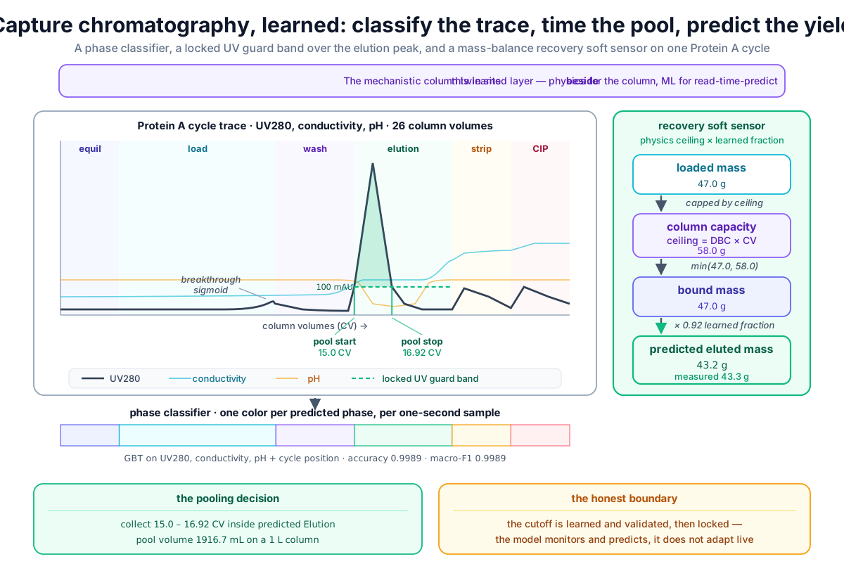Capture, learned: a phase classifier labels every second of the trace, a locked UV guard band over the elution peak picks the pool start and stop on the rising and falling edges, and a mass-balance-anchored soft sensor predicts the recovered mass — the machine-learning layer that sits beside, not instead of, the mechanistic column twin. Original diagram by the authors, created with AI assistance.

Building it: phase classification plus pooling and recovery

The runnable module frames two tasks on one real chromatogram. First, a phase classifier: label each one-second sample as one of the six phases from the three live signals — UV280, conductivity, pH — plus light temporal context. The model is a gradient-boosted tree classifier (the tabular tree-ensemble learner from the model-ladder chapter, which grows many small decision trees in sequence, each correcting the errors of the ones before — here GradientBoostingClassifier, 120 stagewise trees of depth 3, seed 2026, the seed just fixing the random draw so the run reproduces) — a deliberately modest, fully-tabular learner whose shallow depth-3 trees are easy to inspect and trivial to lock for GMP. A bare triplet confuses equilibration with wash (both low UV, neutral pH, similar conductivity); what separates them is where you are in the cycle and which way UV is moving, so the feature vector adds the running column-volume position (cv_position), a 30-second rolling UV slope (UV_slope), and rolling means of UV, pH, and conductivity. That slope feature is what tells equilibration's flat baseline from wash's UV decay; the position feature is honest in real time — the cumulative volume delivered is always known — but it is also a strong hint, so the chapter is candid below about not letting the model simply learn the clock.

Second, pooling and recovery: inside the model-predicted elution phase, apply the locked 100 mAU UV guard band to pick the pool start and stop in column volumes, then a mass-balance-anchored soft sensor predicts the recovered mass. The recovery model encodes the physics ceiling — eluted mass cannot exceed what the column bound, which is the lesser of the mass loaded and the capacity (DBC times column volume) — and lets a recovery fraction fill the gap: the predicted eluted mass is the bound mass — the lesser of the loaded mass and DBC times column volume — multiplied by that recovery fraction. This is a miniature hybrid: physics sets the ceiling, data fills the fraction. One honest caveat about the fraction: in the public single-cycle dataset the 0.92 recovery fraction is read straight from the cycle summary rather than fit, so the 43.2-versus-43.3-g agreement is an identity check (n=1) that demonstrates the hybrid's structure, not a held-out fit; across a multi-cycle dataset the fraction is fit and the prediction becomes a genuine soft sensor.

The two learning tasks are split cleanly in the source — train_phase_classifier() does a 70/30 stratified split (70 percent of samples to train on, 30 percent set aside, with each phase represented in both halves) and reports held-out accuracy (the score on the set-aside rows the model never saw while fitting, on a 0-to-1 scale where 1.0 is perfect) and macro-F1 (a per-class-averaged accuracy score that does not let the model coast on the common phases); predict_pool() re-runs the classifier over the full trace and applies the guard band inside predicted elution; recovery_model() reads the one-row cycle summary and computes the mass-balance prediction. The classifier code is reproduced below verbatim from examples/platform/ml/chromatography.py:

# examples/platform/ml/chromatography.py — phase classifier + pooling/recovery.
import pandas as pd
from sklearn.ensemble import GradientBoostingClassifier
from sklearn.model_selection import train_test_split
from sklearn.metrics import accuracy_score, f1_score

POOL_THRESHOLD_mAU = 100.0   # locked UV guard band for collection
CV_ML = 1000.0               # 1 L Protein A column

def featurize(df):
    f = pd.DataFrame()
    f["UV280"], f["cond"], f["pH"] = df["UV280_mAU"], df["conductivity_mS_cm"], df["pH"]
    f["cv_position"] = df["volume_CV"]                          # where in the cycle (CV elapsed)
    f["UV_slope"] = df["UV280_mAU"].diff().rolling(30, min_periods=1).mean().fillna(0.0)
    f["UV_roll"] = df["UV280_mAU"].rolling(30, min_periods=1).mean()
    f["pH_roll"] = df["pH"].rolling(30, min_periods=1).mean()
    f["cond_roll"] = df["conductivity_mS_cm"].rolling(30, min_periods=1).mean()
    return f

df = pd.read_csv("examples/datasets/protein_a_chromatogram.csv").sort_values("time_s")
X, y = featurize(df).to_numpy(), df["phase"].to_numpy()
Xtr, Xte, ytr, yte = train_test_split(X, y, test_size=0.3, random_state=2026, stratify=y)
clf = GradientBoostingClassifier(n_estimators=120, max_depth=3, random_state=2026).fit(Xtr, ytr)
pred = clf.predict(Xte)
print(f"accuracy={accuracy_score(yte, pred):.4f} macro-F1={f1_score(yte, pred, average='macro'):.4f}")

# real-time pooling: collect inside predicted Elution while UV stays above the guard band
phase_hat = clf.predict(featurize(df).to_numpy())
elute = df[(phase_hat == "Elution") & (df["UV280_mAU"] >= POOL_THRESHOLD_mAU)]
start_cv, stop_cv = float(elute.volume_CV.iloc[0]), float(elute.volume_CV.iloc[-1])
print(f"pool {start_cv}-{stop_cv} CV = {(stop_cv - start_cv) * CV_ML:.1f} mL")

Running it on the simulator's golden capture cycle gives the verified output:

Phase classifier (GBT on UV/cond/pH + context): accuracy=0.9989 macro-F1=0.9989 (2184 train / 936 test samples)
Real-time pooling (UV280 >= 100 mAU in predicted Elution): collect 15.0-16.92 CV, pool 1916.7 mL
Recovery soft sensor: loaded 47.0 g, capacity 58.0 g, bound 47.0 g x 0.92 = 43.2 g (measured 43.3 g)
ASSERT ok: phase classifier recovers the chromatogram structure (accuracy > 0.9).

The classifier recovers the six-phase structure nearly perfectly — accuracy 0.9989 and macro-F1 0.9989 on 936 held-out samples after training on 2184 — the pool window (collect from 15.0 to 16.92 CV for a 1916.7 mL pool) matches the cycle summary in protein_a_summary.csv exactly, and the recovery soft sensor predicts 43.2 g against a measured 43.3 g (a 47.0 g load against a 58.0 g column capacity, so the bed binds all 47.0 g and a 0.92 recovery fraction does the rest). Macro-F1 matters more than raw accuracy here because the six phases are imbalanced — load and elution dominate the sample count while strip and CIP are short — and a macro-average refuses to let the model coast on the majority phases. The near-perfect score is partly because the cycle-position feature is so informative on a single, well-separated cycle; on a real multi-cycle, multi-resin-lot dataset the score would be lower and the classifier would have to lean harder on the signal shape — which is the honest caveat the unsolved section opens with.

Anatomy of one pooling decision

A pooling decision is small — a start, a stop, a pool — but it carries the whole logic of the capture step, and it is worth unpacking one field by field. The record below is the decision the module made on PApool-001, and every field is either a live signal, a learned/locked rule, or a physics-anchored prediction, with nothing invented.

One pooling decision, fully unpacked: three live signals feed a phase classifier that says "Elution," a locked UV guard band picks start and stop on the peak edges, a mass-balance ceiling caps the recoverable mass, and a learned fraction predicts the yield — the lineage from clarified harvest to capture pool carried in a single reviewable record. Original diagram by the authors, created with AI assistance.

Read top to bottom, the record is the chapter in miniature, and each field earns its place:

• Cycle / source — PApool-001, drawn from protein_a_chromatogram.csv (the 3120-sample golden cycle) and protein_a_summary.csv (the one-row decision). This is the identity that the genealogy carries forward.
• Live signals — UV280 (mAU), conductivity (mS/cm), and pH, sampled each second. These are the only inputs available the instant the decision is made; there is no offline assay in the loop, which is the whole point of a real-time rule.
• Predicted phase — the gradient-boosted classifier's call, Elution, with its 0.9989 held-out accuracy. This field gates everything below it: the guard band only applies inside elution, so a UV bump during wash never triggers collection.
• Rule (locked cutoff) — the 100 mAU UV280 guard band, fixed at validation, not adapted live. pool_start 15.0 CV is where the rising edge first crosses 100 mAU; pool_stop 16.92 CV is where the falling edge last crosses it; the difference, 1.92 CV on a 1 L column, is the 1916.7 mL pool.
• Physics ceiling — the mass balance. mass_loaded 47.0 g against column_capacity of DBC 58 g/L × 1 L = 58.0 g, so bound = min(47.0, 58.0) = 47.0 g: the bed had headroom and captured everything it was given. No learning can claim more eluted mass than this.
• Learned fraction — recovery_frac 0.92, the one quantity the physics does not pin down, giving eluted_pred = 47.0 × 0.92 = 43.2 g against a measured 43.3 g. The gap between physics ceiling (47.0) and prediction (43.2) is exactly the resin-and-conditions loss the data has to supply. (On this public single-cycle dataset the 0.92 is read from the cycle summary, so the 43.2-vs-43.3 match is an identity check; across a multi-cycle dataset the fraction is fit and the prediction becomes a held-out soft sensor.)
• Lineage — PApool-001 derivedFrom CLAR-001, the clarified-harvest input from the previous chapter, the same provenance edge carried in the Book 4 genealogy.
• Governance — the cutoff is locked design-time and the model's runtime role is monitoring, not autonomy, consistent with draft Annex 22.

The whole record is auditable after the fact — you can hold the pool the model chose against the assay of what it actually collected, field by field — which is precisely why this pattern passes GMP review where an autonomous controller would not. This is the six-field, self-describing record from Book 2's data-point lifecycle, here carrying a live signal, a locked rule, and a prediction instead of a lab assay — a contextualized record being the unit of audit.

What makes the record machine-checkable: typed triples, a SHACL gate, and a walkable lineage

The card above is a readable summary; underneath it the same facts are typed triples (the subject-predicate-object statements a knowledge graph is made of), which is what lets a machine — not just a reviewer — check the decision. Every field maps onto the ontology Book 4 builds: the three live channels are unit-bearing datatype properties (bp:uv280, bp:conductivity, bp:pH, each carrying a UCUM unit code so mAU and mS/cm are concepts a reasoner relates, not bare spellings on a column header), PApool-001 is a bp:CapturePool from the class taxonomy, and Elution is one of the controlled phase terms rather than a free-text string. The payoff is that the pooling model reads its inputs by IRI, not by column name: the UV channel is the value on bp:uv280 of this cycle, so a renamed or re-ordered CSV export cannot silently mis-feed it — the same brittleness-to-robustness move the MLOps chapter makes for every feature, and the cross-system identity the data book's semantic-interoperability chapter exists to supply.

That identity also tells you which plant systems each field came from, because the graph anchors to the standards the floor already speaks: the live UV/conductivity/pH stream arrives over OPC UA (the vendor-neutral industrial-data transport), the cycle is a batch step in an ISA-95 equipment-and-material hierarchy (IEC 62264 — the model that says which column, on which skid, in which campaign), and the cycle summary is exchangeable as a B2MML batch record (the XML serialization of ISA-95). So the timestamp-alignment and missing-value rules a data engineer worries about are not ad-hoc: a sample is keyed to its OPC UA source timestamp, a dropped second is a gap the graph can see rather than a row silently shifted, and the one-per-second cadence is a property of the equipment record, not a guess from row order.

The closed-world check is the load-bearing part. Before this cycle's record is allowed to train or re-validate the pooling model, it is validated against a SHACL shape (the Shapes Constraint Language — a closed-world rule that every required field be present, singular, typed, and in range), the very same discipline the release gate uses to decide whether a lot may ship. The question SHACL answers — is a required result missing? — is one no SELECT query can pose, because it is about the triples that should exist and do not; pointed at a training row instead of a release lot, that shape guarantees every cycle carries its UV trace, its loaded mass, its measured recovery, and its lineage edge before a single fit, so a half-built record is refused at the gate rather than discovered three folds into cross-validation. And the lineage field is not decoration: PApool-001 bp:derivedFrom CLAR-001 is a PROV-O provenance edge (the W3C provenance vocabulary the genealogy chapter builds the digital thread from, aligned to the OBO Relation Ontology's derives from), and that transitive edge is exactly the grouping key the leave-one-cycle-out validation below needs — whole-cycle (and whole-resin-lot) groups are defined by walking the lineage IRI as a SPARQL traversal, not by trusting a coincidental cycle_id column. The BFO continuant/occurrent cut keeps the last piece honest: the recovered-mass measurement (a continuant quality of the pool) is a distinct thing from the capture cycle (an occurrent) that produced it, so the soft sensor never conflates the number with the run that made it.

One layer makes that record legally sufficient rather than merely tidy. Because the pooling decision can steer a CQA-affecting operation, it is a regulated electronic record: every field must satisfy ALCOA+ (Attributable, Legible, Contemporaneous, Original, Accurate — plus Complete, Consistent, Enduring, Available) — attributable to the locked model version that chose the cutoff, contemporaneous because each sample is timestamped as it streams, and Complete because the SHACL gate above refuses a record with a missing field — and the locked cutoff, the model version, and the disposition carry the attributable electronic signature and immutable audit trail that 21 CFR Part 11 (US) and EU GMP Annex 11 (EU) require of electronic records and signatures. The sh:minCount 1 on the approval field is the SHACL spelling of "an unsigned release is no release," so the ontology obligation and the Part 11 obligation are the same obligation in two layers — which is why a pooling record assembled this way is admissible in front of an inspector and a spreadsheet export of the same numbers is not.

The unsolved part: capacity drift, resin lifetime, and the locked-model paradox

The hard, unsolved problem in capture is time — specifically, that the column is not the same column on cycle 200 as on cycle 1. Protein A resin is expensive and is validated for a finite cycle life; over that life its dynamic binding capacity slowly falls, its back-pressure rises (the bed resists flow more as it fouls and compacts, so pushing liquid through takes more pressure), the breakthrough front smears, and its impurity clearance can drift. A model that perfectly times the pool today will, if frozen, slowly mistime it as the resin ages and the peak shape shifts — the elution peak broadens and shoulders, the 100 mAU crossings move, and a fixed guard band starts clipping or over-collecting. This is the model decay problem this book keeps meeting, here driven by a physical asset wearing out rather than by a biological process drifting, which makes it both more predictable (aging is monotone) and more inescapable (you cannot reset the resin).

This collides head-on with the regulatory reality, and the collision is the genuinely unsolved part. The very fix a data scientist wants — let the model adapt to the aging resin, nudging the cutoff cycle by cycle — is the thing draft Annex 22 most explicitly forbids for a critical GMP function: it requires locked deterministic models and a predetermined change-control plan, not online adaptation. So the field is left with an awkward middle ground that nobody has fully solved at scale: detect the drift (the resin-aging monitors — PCA on chromatographic features, hybrid lumped-kinetic aging models, moment analysis — are good at this), but respond to it through governed retraining and validated cleaning/re-equilibration cycles, not through a model quietly rewriting its own pooling rule. Doing that well means answering three open questions: when has a model decayed enough to warrant a controlled retrain (a drift-detection threshold that is itself a validated artifact); how do you prove the retrained model is at least as safe as the locked one it replaces (the equivalence argument); and who signs off — a change-control loop that may take longer than the resin has cycles left. This is the open MLOps problem of downstream, and it is genuinely unsolved at scale.

A second unsolved piece is the one our own demo exposed: the phase classifier leaned heavily on cycle position, and a single clean cycle made that trivially easy. Real capture data is multi-cycle, multi-resin-lot, multi-scale, and the genuinely hard version of phase detection — robust to a column that channels, a feed that is off-spec, a pump that stutters, a cycle that is paused and resumed so the volume clock no longer aligns with the trace shape — is much harder than 0.9989 accuracy on one golden run suggests. Distinguishing learning the signal from learning the clock is the difference between a classifier that generalizes to a fouled column and one that memorizes the schedule and fails the moment the schedule slips. There is a subtler leak in the same demo: the rolling-window features are computed over the whole trace before the split, so every held-out sample shares its 30-second window with up to twenty-nine training samples — the random split is not even clean at the feature level, the feature-leakage and grouped-split discipline the data chapter sets out. (That sharing is "cheating" because a test sample is supposed to be genuinely unseen; if it was averaged together with its training neighbours, the model has effectively already met it.) An honest validation therefore withholds whole cycles (and whole resin lots), not random samples within one cycle — leave-one-cycle-out (hold back every sample from one whole cycle as the test set), not a stratified split (which scatters samples from the same cycle across both train and test) — and recomputes the windowed features inside each fold so no test sample borrows context from a training neighbour; the score on that protocol is the number that would actually predict plant behaviour.

What this chapter adds to the model suite

This chapter contributes examples/platform/ml/chromatography.py to Book 5's example suite — the Protein A phase classifier plus the pooling-and-recovery model. It provides:

• train_phase_classifier() — a gradient-boosted six-class phase classifier over UV280, conductivity, pH, and temporal context (cycle position, 30 s rolling slope and means), validated on a 70/30 stratified held-out split of the real chromatogram (accuracy 0.9989, macro-F1 0.9989; 2184 train / 936 test samples).
• predict_pool() — the real-time pooling rule: the locked 100 mAU UV guard band applied inside the model-predicted elution phase, returning start/stop column volumes (15.0–16.92 CV) and pool volume (1916.7 mL) that match the cycle summary.
• recovery_model() — the mass-balance-anchored recovery soft sensor: a physics ceiling (the lesser of loaded mass and DBC times column volume, 47.0 g of a 58.0 g capacity) times a learned recovery fraction (0.92), predicting 43.2 g against a measured 43.3 g.

It reads examples/datasets/protein_a_chromatogram.csv (3120 one-second samples) and protein_a_summary.csv (the cycle's pooling decision and recovery), and it deliberately complements rather than duplicates the upstream soft sensors — soft_sensor_pls.py and hybrid_model.py — by working on a downstream unit operation with a categorical (phase) task alongside the regression.

Why it matters

Capture sets the impurity floor for the entire purification train, and the pooling decision it makes — live, on a moving signal — is one of the few places in manufacturing where a model's choice has an immediate, measurable, auditable consequence on product quality and yield. Getting the learning layer right means three concrete things: a phase classifier that automates chromatogram review so a human reviews exceptions, not every trace; a pooling rule that is learned and validated but locked, trading yield against purity on evidence rather than on a fixed historical window; and a recovery soft sensor that tells the operator the yield before the assay does. Get the boundary right — mechanistic physics for the column, machine learning for read-time-predict, neither pretending to be the other — and capture becomes the model citizen of downstream ML: real, deployed-adjacent, and honest about its limits. Blur the boundary, call a solved-physics simulator "AI," or let a model adapt its own CQA-affecting rule, and you have either over-claimed or stepped over the line the regulators have drawn brightest. The golden cycle BATCH-2026-001 carries a 98.611 percent monomer (the single, correctly-folded antibody — the desired form, as opposed to the high-molecular-weight aggregate clumps) through this step on the strength of exactly that discipline.

In the real world

Mechanistic chromatography modeling is production technology in CMC process development: Cytiva GoSilico and the open-source CADET are used to model elution and breakthrough for real molecules, and disclosed industrial groups have built mechanistic ion-exchange and mixed-mode models in their pipelines [1][2] — maturity: production, but, again, this is mechanistic, not ML, and vendor savings headlines are vendor-self-reported. On the learning side, the deployed-adjacent reality is monitoring and prediction rather than autonomous control, and it sorts cleanly by maturity:

• Pilot, named deployment. ML-based Raman has been used to predict 16 quality attributes in-line during Protein A capture — a pilot at Boehringer Ingelheim (Late Stage Downstream Process Development, with Karlsruhe Institute of Technology), using a k-nearest-neighbours regressor on Butterworth-filtered spectra, explicitly not a deep-learning model, a point worth correcting wherever it is miscited [8].
• Pilot. On-line PAT plus PCA has flagged Protein A resin aging 20–25 cycles ahead of yield loss [6].
• Research. PINN-accelerated mechanistic models have reached real-time speeds (offline fit 2608.6 s to 110.7 s; online 12 to 14 s) for model-predictive control of continuous 4C-PCC capture [5]; and CNN-guided Raman has made charge-variant pooling calls on a CEX polishing step at R-squared 0.94 to 0.99 (the polishing result discussed above).

The pattern matches the ISPE Pharma 4.0 picture the whole book reports: downstream ML clusters in monitoring, prediction, and human-in-the-loop review — not in autonomous control of a critical quality attribute. The open-source analytics chapter shows the same shape of model running in code, and Book 1's capture chromatography and Book 4's downstream ontology describe the same physical step through their own lenses.

Key terms

• Capture (Protein A) chromatography — the first downstream step, a bind-and-elute cycle that removes most impurities and concentrates the antibody several-fold, yielding the capture pool PApool-001.
• Phase — one of the six segments of a capture cycle (equilibration, load, wash, elution, strip, CIP), each with a distinct UV-conductivity-pH signature; classified per-sample from the live signals.
• Breakthrough — antibody escaping the column unbound when the resin saturates during load; the rising outlet UV sigmoid that marks it bounds how much can be loaded.
• Dynamic binding capacity (DBC) — the mass the column can hold at the operating flow before a fixed breakthrough level (often 10 percent, DBC10); not a constant — it falls as the resin ages and shifts with flow rate, temperature, and titer.
• General rate model (GRM) — the first-principles column PDE system: convection-dispersion in the bulk, film transfer and pore diffusion into the beads, closed by a binding isotherm; the backbone of mechanistic chromatography simulation.
• Steric mass action (SMA) — the ion-exchange isotherm in which protein competes with salt counter-ions for sites under characteristic charge and steric shielding; pairs with the GRM in GoSilico and CADET.
• Pooling decision — choosing the start and stop of eluate collection, typically as a guard band on UV280 (and sometimes conductivity or pH), trading recovery against purity; in production the cutoff is learned and validated but locked, not adapted live.
• Mechanistic chromatography model — a first-principles column simulator (GRM + SMA; GoSilico, CADET); the mature production tool here and not machine learning.
• Hybrid (gray-box) chromatography model — a mechanistic backbone whose hard-to-measure parameters (serial) or residuals (parallel) are supplied by a learned component; the small-data-friendly middle path.
• Recovery soft sensor — a prediction of eluted mass from a physics ceiling (the lesser of loaded mass and DBC times column volume) times a learned recovery fraction.
• Feature by IRI — wiring the pooling model's inputs to semantically identified, unit-bearing quantities (bp:uv280 and friends, with UCUM units and BFO typing) instead of fragile column names, anchored to the ISA-95 / OPC UA / B2MML standards the plant systems already speak, so a renamed or re-ordered export cannot silently mis-feed it.
• SHACL-validated training record — running the same closed-world release-gate shape (bp:ReleaseShape: every required field present, singular, typed, in range) over a cycle's record before it trains or re-validates the pooling model, so a half-built record is refused at the gate, not discovered three folds into cross-validation.
• bp:derivedFrom / PROV-O lineage — the transitive provenance edge (PApool-001 derivedFrom CLAR-001, aligned to the OBO Relation Ontology's derives from) carried in the digital thread; the grouping key that makes leave-one-cycle-out validation honest, walked as a SPARQL traversal rather than trusting a cycle_id column.
• ALCOA+ / 21 CFR Part 11 / EU Annex 11 — the data-integrity standard and the electronic-records-and-signatures rules a CQA-affecting pooling record must meet: an attributable model version, a contemporaneous timestamp, a complete (SHACL-gated) record, and an immutable audit trail with a signed disposition.

Where this leads

The capture pool PApool-001 is concentrated, low-pH, and far purer than the harvest — but "far purer" is not "safe." Before the product can advance, the process must prove it can clear viruses by a validated margin, and that proof is a number with a hard floor. The next chapter, Viral Safety: Learning Log-Reduction and Orthogonal Clearance, takes up the log-reduction-value problem — how learning predicts and supports viral clearance across orthogonal steps, and why this is the most safety-critical place in the whole book to be careful about what a model is allowed to claim.