Cell-Line Development: Ranking Clones with Machine Learning

📍 Where we are: Part II · Discovery & Development, Learned — Chapter 6. The previous chapter, Molecule Discovery, used generative design and developability prediction to choose what protein to make. Now we choose which cell will make it — and we do it under the same small-data, high-stakes pressure, only with thousands of candidate clones instead of millions of candidate sequences.

Cell-line development (CLD) is where a sequence on a screen becomes a living factory. A pool of CHO cells (Chinese Hamster Ovary cells, the standard mammalian host for antibody manufacturing) is transfected with the gene for mAb-A (the monoclonal antibody — mAb — this series follows) — that is, the mAb-A gene is inserted into the cells' DNA — the survivors are diluted to single cells, and each surviving cell grows into a clone — a population descended from one founder. Out of thousands of clones, a handful will become candidates for the master cell bank (the archival parent stock the line is frozen from), and exactly one lineage will become WCB-CHO-001, the working cell bank (the everyday vials drawn from the master bank to seed each batch) that seeds every commercial batch in this book. The choice is irreversible in the way few decisions are: a clone selected here is locked into the process development, the production bioreactor, and the release specification for the life of the product. Pick a clone that grows fast but drifts genetically, or one that titers high (produces a lot of antibody — the titer is the concentration of antibody the cells make, in grams per litre) but makes the wrong glycoform (the wrong pattern of sugar structures on the antibody — more on this below), and the cost surfaces years and hundreds of millions of dollars downstream.

The traditional way to choose is to grow every promising clone all the way to a 14-day fed-batch shake-flask or mini-bioreactor run (a fed-batch run feeds the culture nutrients over its ~two-week lifetime rather than starving it after one charge — the standard productivity screen), assay the titer and quality, and rank. That is slow, expensive, and — the part machine learning attacks — late. Most of the screening budget is spent on clones that a model could have flagged as losers in week one. This chapter reframes clone selection as a learning-to-rank problem: learn, from cheap early signals, the order in which clones will finish, and spend the expensive late assays only on the top of the predicted ranking.

The simple version

Imagine scouting a thousand young athletes when you can only sign a dozen. You cannot run a full season for each. So you measure cheap early signals — sprint time, vertical jump, how their numbers trend over a few weeks — and you learn, from athletes you scouted in past years and then watched play, which early signals actually predict a good career. A clone-ranking model does the same for cells: it watches cheap early signals (how fast a clone grows, what it looks like under a microscope, how its lactate trends) and learns, from past clones whose full 14-day outcome you already know, which ones are worth the expensive late screen.

The key word is learn: the model only works because, for thousands of clones from past campaigns, you eventually saw the full 14-day result. Those finished clones are the training set.

The twist the rest of this chapter develops: a good scout does not sign the fastest sprinter — they sign the athlete who is fast and durable and coachable. A titer-only screen signs the sprinter. A multi-attribute ranker signs the player.

What this chapter covers

We treat clone selection as a supervised learning-to-rank task layered on top of a few classification and regression sub-models. We cover: the imaging problem (high-content, often label-free microscopy plus an ML classifier for clonality assurance and clone health); the feature problem (turning sparse growth curves, metabolite trajectories, and omics readouts into a fixed feature vector per clone); the manufacturability index that fuses titer, quality, and stability predictions into one ranking score; the early stability prediction that tries to call genetic and titer stability long before a months-long stability study finishes; and the GMP (Good Manufacturing Practice — the regulated commercial-manufacturing regime) and-genealogy angle that ties the chosen clone to WCB-CHO-001. The runnable artifact is examples/platform/ml/clone_rank.py, which ranks a synthetic clone panel from early features and — the chapter's central empirical claim — shows a multi-attribute ranker beating a titer-only screen.

The task: clone selection is learning-to-rank, not regression

It is tempting to frame CLD as "predict each clone's final titer, then sort." That is a pointwise regression framing, and it is the wrong one for two reasons. First, the absolute titer of a clone is not what you act on — its rank relative to its siblings in the same campaign is, because you advance the top-k regardless of the absolute numbers, and campaign-to-campaign offsets (a different transfection efficiency, a different operator, a different media lot) shift every clone together without changing who wins. Second, the loss you actually care about is concentrated at the top of the list: getting the rank order right among the top 20 clones matters enormously; getting it right among the bottom 800 is irrelevant, because none of them advance.

This is exactly the setting learning-to-rank was built for. The three classic families are pointwise (predict each clone's score independently, then sort — simple, but blind to the relative structure), pairwise (learn, for each pair of clones, which one should rank higher — the objective LambdaMART and RankNet optimize), and listwise (optimize a whole ranking metric directly). The pairwise objective is the most natural fit: define, for an ordered pair (i, j) where clone i truly outranks clone j, a model score s(·), and minimize the logistic pairwise loss

L_pair = Σ_(i>j)  log( 1 + exp( -( s(x_i) − s(x_j) ) ) )

which simply pushes the predicted score of the better clone above the worse one for every comparable pair. LambdaMART weights each pair by how much swapping it would change a ranking metric, so it spends gradient where the ranking metric is most sensitive — the top of the list. The metric that matches CLD's "top of the list is what matters" reality is NDCG@k (normalized discounted cumulative gain at rank k):

DCG@k  = Σ_(r=1..k)  gain(clone at rank r) / log2(r + 1)
NDCG@k = DCG@k / IDCG@k     (IDCG@k = DCG of the ideal ordering)

The 1/log2(r+1) discount means a good clone surfaced at rank 2 counts for far more than one buried at rank 40, which is precisely the economics of a screen that advances ~20 clones. A model whose NDCG@20 is high will surface the right clones into the expensive screen even if its absolute titer predictions are mediocre — and that is the only thing the wet lab cares about.

In practice, two pragmatic framings dominate the small-data CLD regime, and the worked example below uses the second. The first is a gradient-boosted tree (a GBDT such as XGBoost or LightGBM) trained directly with rank:pairwise / LambdaMART. The second — robust when clone counts are in the low hundreds and labels are coarse — is to recast "advance or not" as a binary classification of good manufacturing clone vs not, fit a classifier, and rank by its predicted probability; ranking by P(good) is itself a valid pointwise ranker, and its AUROC is exactly the probability that a randomly chosen good clone outscores a randomly chosen bad one — a ranking quality metric in disguise. Note that for ranking the classifier need not be calibrated (its scores need not match true probabilities), only monotone in P(good) (it must merely put better clones above worse ones): AUROC and the rank order are invariant to any monotone transform of the score, so a raw predict_proba that orders clones correctly is enough, and the worked example below leans on exactly that. The deeper point holds either way: the model's job is to allocate the screening budget, not to replace the screen. The final titer and quality numbers still come from a real 14-day run on the surviving candidates. The model decides which clones earn that run.

The features: cheap early signals, and the cold-start that bites here too

A clone-ranking model is only as good as the features it can compute early and cheaply, because the entire value proposition is acting before the expensive late assay. The feature families, roughly in order of how early they become available:

• Imaging features. From day one, each well can be imaged. Classical features are confluence, colony morphology, well-occupancy, and per-colony shape descriptors (area, circularity, solidity); modern features are learned embeddings from a CNN or a label-free multimodal microscope (more on this below). Imaging answers two questions at once: is this well truly clonal (a regulatory must), and does this clone look healthy and well-shaped.
• Growth-curve features. Sparse viable-cell-density (VCD) readings — in this book's data, the offline assays sampled roughly twice a day in examples/datasets/offline_assays.csv — are fit to a growth model, and the parameters of that fit become features rather than the raw points. A standard choice is the logistic form fit by nonlinear least squares, VCD(t) = K / (1 + exp(−mu_max·(t − t0))), from which fall out the logistic rate parameter mu_max (the specific growth rate in the exponential phase), the integral of viable cells (IVCD = ∫ VCD dt, a proxy for total biosynthetic capacity), the carrying-capacity asymptote K (a proxy for peak VCD), and the day the culture peaks. (The Gompertz curve is an alternative asymmetric sigmoid whose mu_max relates to its own parameters differently; only the logistic is displayed here.) Fitting parameters rather than feeding raw sparse points both denoises the measurement and gives the downstream model a fixed-length, interpretable vector regardless of how many timepoints a given clone happened to get. A clone's growth shape in the first few days is more predictive than any single VCD point.
• Metabolic features. The same sparse offline panel carries glucose, lactate, glutamine, ammonia, and osmolality. The single most informative derived feature is the lactate trajectory — specifically whether and when a clone switches from producing lactate to consuming it (the "lactate shift"). Operationally it is the day the sign of d[lactate]/dt flips from positive to negative; a clone that never shifts is encoded as a sentinel (e.g. −1). A clone that keeps accumulating lactate is metabolically inefficient, acidifies its own culture, and tends to titer poorly; the shift is a well-established health signal. Mechanistically, the shift to lactate consumption marks a move from glycolytic overflow toward oxidative (TCA) metabolism, which sustains viability at high cell density and reduces the base addition (and osmolality rise) that lactate accumulation forces — which is why a clone that shifts early tends to titer well.
• Early productivity. A day-3 or day-5 titer (even a crude Protein A or biolayer-interferometry reading) is a weak but real early predictor of final titer, and specific productivity (qP, picograms per cell per day) separates a genuinely productive clone from one that is merely growing fast. A useful early proxy is qP ≈ titer / IVCD, normalizing the product made by the cell-days that made it — a clone with modest titer but tiny IVCD is per-cell a star.
• Omics / genetic features. Transgene copy number (how many copies of the inserted mAb gene the clone carries) and integration-site context (where in the genome the gene landed, which governs how reliably it stays switched on), and — where available — transcriptomic markers of stress and the unfolded-protein response. These are the features most predictive of stability, the hardest target, because they speak to whether the clone's productivity will survive 60+ generations of expansion.

Here CLD inherits the cold-start reality that haunts all of bioprocess ML, with its own cruel twist. The label you most want to predict — clone stability over a long-term passaging study — takes months to observe, so your training set of (early-features → confirmed-stable) pairs grows agonizingly slowly, and every label is a clone you already invested a full study in. You are perpetually short of exactly the examples the hardest sub-model needs. This is why hybrid and transfer-learning approaches, which let knowledge from past molecules and past campaigns carry over, matter as much here as anywhere in the book. The CHO hybrid-modeling thesis line of work [4] (research) is built precisely on this constraint: a multi-clone kinetic model whose mechanistic core describes ~140 CHO lines lets an ML layer predict a new clone's kinetic parameters from early well-plate and T25 screening, forecasting bioreactor behavior from far fewer late-stage runs — borrowing strength across clones to escape the per-clone label famine.

High-content imaging and the clonality problem

Two of the imaging model's jobs are different in kind. One is clonality assurance: regulators (under ICH Q5D — ICH is the International Council for Harmonisation, whose guidelines carry regulatory weight; Q5D covers cell-substrate derivation and characterization) require documented evidence that a production cell line descends from a single cell. The classic evidence is photographic — an image of a single cell in a well on day zero — but human review of thousands of wells is slow and subjective, and ML image classifiers now assist by flagging wells that are probably not monoclonal (two founders, a doublet, debris mistaken for a cell). The model here is typically a CNN trained as a binary classifier on day-0 / day-1 well crops, and the operating point matters more than the accuracy: clonality is a screening problem where the cost of a false "monoclonal" call (advancing a polyclonal line) dwarfs the cost of a false "not monoclonal" (re-imaging or discarding a good well), so the threshold is set for very high recall of non-clonal wells, accepting more manual review to drive misses toward zero.

Crucially, this is a decision-support role, not an autonomous one: a model that says "this well is clonal" does not by itself satisfy the regulatory burden; it triages the queue so human reviewers and orthogonal evidence (imaging at two timepoints, limiting-dilution Poisson statistics) concentrate where they are needed. Clonality itself is established as a documented probability of monoclonality — imaging evidence combined with limiting-dilution Poisson statistics — not absolute proof, which is exactly why an ML image classifier can triage the queue but cannot discharge the regulatory burden. This human-in-the-loop framing — ML triages, humans and orthogonal methods decide — is the recurring shape of every honest production deployment in this book.

The other job is clone-health and productivity prediction from images. The strongest research result here is striking: label-free multimodal nonlinear optical microscopy (SLAM/FLIM — simultaneous label-free autofluorescence-multiharmonic imaging and fluorescence-lifetime imaging) combined with an ML classifier distinguished CHO clones as early as passage 2 (a passage is one cycle of growing the cells and splitting them into fresh vessels — a rough unit of culture age, each passage spanning several cell doublings) with a balanced accuracy above 96.8 percent, without any stains or labels that would disturb the cells destined for production [1] (research). Label-free is the operative word: anything you add to characterize a clone is something you must prove you removed before that clone makes a drug, so a method that reads clone identity and health from the cells' own optical signatures (NAD(P)H/FAD autofluorescence ratios as a redox/metabolic readout, second- and third-harmonic structural signals) is uniquely suited to CLD. A complementary line of work builds a relative-titer predictive model purely from image analysis, extracting quantitative morphology features (size, circularity, solidity) from cell-line-development microscopy and ranking high-producing clones before any titer assay runs [2] (research) — with the honest caveat, reported in that same work, that accuracy degrades when the host cell changes, the classic generalization failure of a morphology model trained on one background.

Evidence

The label-free SLAM/FLIM + ML clone-classification result (balanced accuracy above 96.8 percent at passage 2) is peer-reviewed-independent but (research) — an academic demonstration, not a deployed GMP CLD pipeline [1]. The image-analysis relative-titer model is likewise peer-reviewed and early-stage, and self-reports reduced accuracy on a different host cell [2]. Treat both as evidence of feasibility and direction, not of routine industrial use. The strongest production ML in CLD today is more mundane: imaging-assisted clonality triage and data-lake-driven ranking, not autonomous clone calling.

The manufacturability index: fusing many predictions into one rank

A clone is not chosen on titer alone. The decision is multi-objective: high titer, the right product quality (monomer purity, charge variants, glycosylation), good growth, metabolic efficiency, and — the long pole — stability. The industrial pattern that has reached production is the manufacturability index: a single composite score that fuses these objectives, computed over a data lake that pools every measurement ever taken on a clone across the CLD workflow. The published "CLD 4.0" methodology describes exactly this — a four-step Industry-4.0 workflow that pulls raw CLD data into a data lake, computes a Cell Line Manufacturability Index (MICL) ranking clones across productivity, growth, and product-quality criteria rather than any single attribute, applies ML to flag process and CQA (Critical Quality Attribute) risks, and uses natural-language generation to auto-write the selection report; it was demonstrated on a recombinant CHO antibody-peptide fusion with a trisulfide-bond quality issue [3] (production).

The index is where domain weighting meets learned prediction, and the honest version keeps the two separable. Each component can be a learned prediction (predicted final titer, predicted monomer percent, predicted stability probability), but the fusion into one score is a transparent, documented weighting — because a quality unit must be able to explain why clone A outranked clone B, and "the gradient boosting said so" is not an explanation a regulator accepts. So the practical architecture is: learned sub-models produce calibrated per-objective predictions with uncertainty, and a governed scoring function combines them into the rank. Two fusion forms are common. The simplest is a weighted sum of normalized attributes. The more defensible is a Derringer–Suich desirability function, which maps each attribute to a desirability d_i ∈ [0,1] through a documented target/spec curve and combines them as a geometric mean,

D = ( d_1 · d_2 · … · d_m )^(1/m)

whose key property is that any single d_i = 0 zeroes the whole score — a clone that fails one critical attribute (say, monomer below spec) cannot buy its way back with a spectacular titer. That veto behavior is exactly what a multi-attribute selection wants and what a weighted sum lacks. Either way the weights and target curves are set by the development team and version-controlled. This separation is what makes the index auditable. It also makes it tunable: if a program decides stability matters more than peak titer, you change a weight, not a model.

manufacturability_index(clone) =
      w_titer    · norm(predicted_final_titer)
    + w_quality  · norm(predicted_monomer_pct)
    + w_glyco    · norm(predicted_glycan_score)
    + w_growth   · norm(IVCD)
    + w_metabolic· norm(lactate_shift_score)
    + w_stability· P(stable over 60 generations)
                 − penalty(clonality_uncertainty)

Each norm(...) rescales a predicted attribute to a comparable 0–1 range; each w_* is a documented, version-controlled weight; the stability term is a probability from the hardest sub-model; and the clonality penalty pushes wells with weak monoclonality evidence down the list regardless of how well they titer. The predicted_glycan_score term — kept illustrative here — is included because for an effector-function-relevant IgG the glycoform (afucosylation, high-mannose) is frequently the clone-dependent attribute that disqualifies an otherwise excellent clone; it is exactly the kind of critical attribute a Derringer–Suich desirability function would zero, vetoing the whole score. The output is one number per clone — and, more usefully, an ordering with uncertainty bands, so the team advances the confident top-k plus the high-variance near-misses worth de-risking. Note that the formula block above (and the worked example below) implements the additive weighted sum, the simpler of the two fusion forms — not the geometric-mean desirability the prose calls "more defensible"; the additive sum is shown for legibility, with the desirability veto behavior left as the more rigorous production choice.

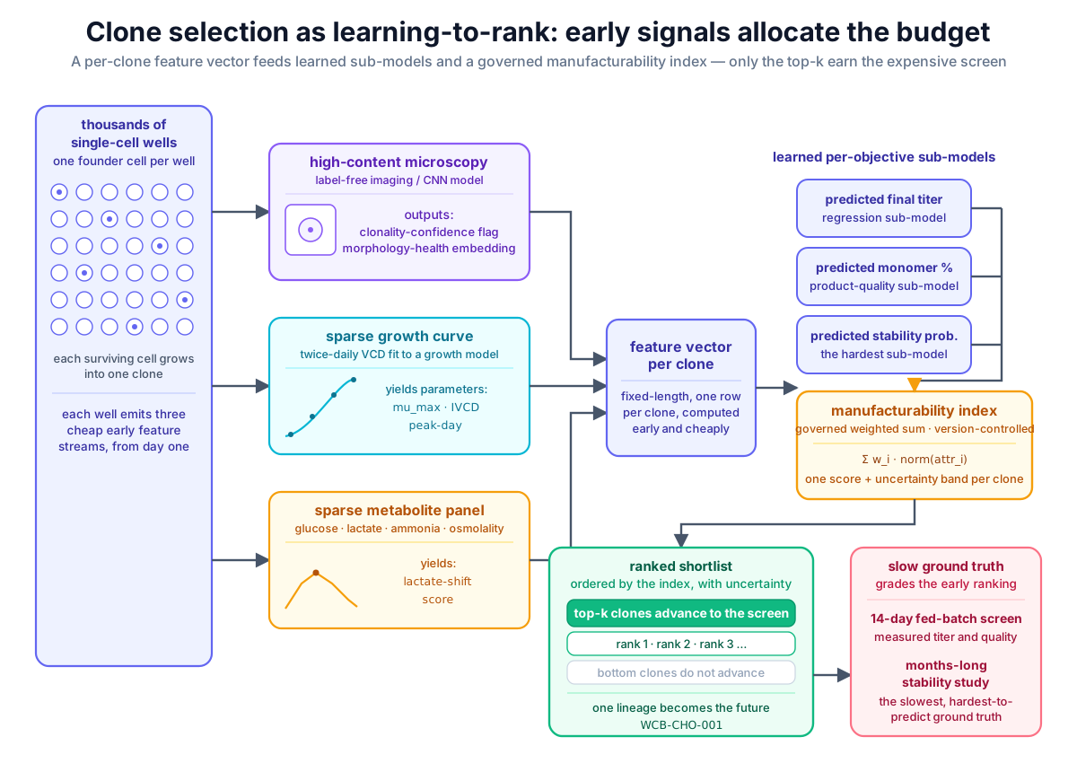Clone selection as budget allocation: cheap early imaging, growth-curve, and metabolic features become a per-clone feature vector, learned sub-models predict each objective, a transparent weighted manufacturability index ranks the clones, and only the top of the predicted ranking earns the expensive 14-day screen that produces the real titer and quality — with the months-long stability study as the slowest, hardest-to-predict ground truth. Original diagram by the authors, created with AI assistance.

Glycosylation: the attribute the clone and the process share

The predicted_glycan_score term in the index above deserves a section of its own, because glycosylation is the clearest example in this book of a quality attribute that no single stage owns. It recurs at every step of mAb-A's life — a sequence liability at discovery, an effector-function veto here in clone selection, a scale-up exposure in process development, and a release attribute in QC — yet the book develops it as a through-line nowhere until now. This section closes that gap.

Glycosylation is the set of branched sugar structures (glycans) attached to a conserved site on an antibody's Fc region. mAb-A is an IgG1, and for an IgG1 the Fc glycan is not cosmetic: it tunes effector function — the antibody's ability to recruit immune killing through ADCC (antibody-dependent cell-mediated cytotoxicity) and CDC (complement-dependent cytotoxicity). The textbook levers are well established by name: afucosylation (removing a core fucose) sharply raises ADCC, and galactosylation modulates CDC; high-mannose and other glycoforms can shorten serum half-life and raise immunogenicity or clearance concerns. That is why glycoform is a genuine CQA and, in clone selection, can be an effector-function veto — exactly the kind of attribute a Derringer–Suich desirability function would zero, sinking an otherwise high-titer clone whose glycan profile is wrong.

The split the attribute forces — and the one worth making explicit — is between its molecule-intrinsic part and its process-and-host-realized part:

• Molecule-intrinsic (predictable early, in silico). Whether the sequence even carries an N-linked glycosylation site is written in the amino acids: an N-X-S/T sequon (asparagine, any residue except proline, then serine or threonine). A developability model at the discovery stage can flag a sequon — especially an unwanted one in a CDR — as a liability directly from the sequence, no cells required. This is the same in-silico-from-sequence regime as the aggregation and immunogenicity liabilities that chapter already screens.
• Process-and-host-realized (only measurable downstream). The actual distribution of glycoforms — how much is afucosylated, how much is high-mannose — is not in the sequence. It is realized by the living system: the CHO clone's own glycosylation machinery, the media, the pH, the feed strategy, and dissolved-gas conditions in the bioreactor all shift it. A model can promise that a sequon is present or absent; it cannot promise the realized glycoform. That needs the process.

The practical consequence runs straight through this chapter's argument. An in-silico model flags sequon liability at discovery, but the realized glycoform is a clone-dependent attribute that only a real culture reveals — which is why it lives as a per-objective sub-score in the manufacturability index, vetoing a clone the molecule alone could never disqualify.

Learning the realized glycoform is hard for the same reason stability is. Glycan profiles are multi-attribute compositional data (the fractions of many glycan species that sum to a whole) read out by slow, specialized analytics — released-glycan HPLC or mass spectrometry — so they arrive scarce, a handful of measurements per batch rather than a dense stream. That is the small-data ceiling again, in its compositional form: too few labeled glycoform readings to train a model that could replace the assay. So glycan ML, like clonality and stability ML in this chapter, plays a triage-and-monitor role — flagging clones and conditions whose glycoform is likely off-target and worth an early intensive check — not a release role. The released-glycan assay still has the last word, exactly as the 14-day titer run does for productivity.

A worked ranker: multi-attribute learning beats a titer-only screen

The companion module examples/platform/ml/clone_rank.py makes the central claim concrete and falsifiable: a learned multi-attribute ranker outranks a titer-only screen at finding the clones worth advancing. There is no public multi-thousand-clone CLD dataset to ship, so the module synthesizes a plausible 240-clone screen whose attributes correlate with a hidden multi-attribute truth, then fits a ranker on the early features and compares it head-to-head against ranking by titer alone. Every number is from the synthetic generator, but the structure of the comparison is the real lesson, and the gap it produces is the whole argument for the manufacturability index.

The simulator gives each clone five measured early attributes — final titer (g/L), specific growth rate (1/day), an aggregation / high-molecular-weight quality readout (HMW % — the fraction of antibody that has clumped into larger-than-monomer species, an undesirable quality defect), an early stability-drop estimate (% titer lost by generation 60), and a crude specific-productivity proxy. Then it defines the hidden truth a titer-only screen cannot see: a clone is "good" only if it is high-titer and low-aggregation and stable. That is the manufacturability index in miniature — a multi-attribute label — and the experiment asks whether a classifier trained on all five attributes recovers it better than sorting on titer.

# examples/platform/ml/clone_rank.py  (excerpt) — rank clones by a learned
# manufacturability score, and beat a titer-only baseline.
import numpy as np
from sklearn.ensemble import RandomForestClassifier
from sklearn.metrics import roc_auc_score
from sklearn.model_selection import train_test_split

N = 240

def make_clones(seed=2026):
    rng = np.random.default_rng(seed)
    titer = rng.normal(4.5, 1.2, N).clip(0.5, 9)              # g/L
    growth = rng.normal(0.55, 0.08, N)                        # 1/day
    aggregation = rng.normal(2.0, 1.1, N).clip(0.1, 8)        # HMW %
    stability_drop = rng.normal(8, 5, N).clip(0, 30)          # % titer loss by gen 60
    spec_prod = titer / (growth * 14)                         # crude qP proxy
    X = np.column_stack([titer, growth, aggregation, stability_drop, spec_prod])
    # "good" = high titer, low aggregation, stable — a multi-attribute truth a
    # titer-only screen cannot see.
    score = (titer / 9) - 0.6 * (aggregation / 8) - 0.5 * (stability_drop / 30)
    good = (score > np.quantile(score, 0.7)).astype(int)
    return X, good, titer

def main() -> dict:
    X, good, titer = make_clones()
    Xtr, Xte, ytr, yte, _, titer_te = train_test_split(
        X, good, titer, test_size=0.35, random_state=0, stratify=good)
    clf = RandomForestClassifier(n_estimators=300, random_state=0)
    clf.fit(Xtr, ytr)
    proba = clf.predict_proba(Xte)[:, 1]
    auroc = roc_auc_score(yte, proba)
    auroc_titer = roc_auc_score(yte, titer_te)           # baseline: rank by titer alone
    top5 = np.argsort(proba)[::-1][:5]                   # of advanced clones, how many good?
    top5_precision = yte[top5].mean()
    print("Clone manufacturability ranking (synthetic 240-clone screen)")
    print(f"  learned ranker AUROC = {auroc:.3f}  (titer-only baseline AUROC = {auroc_titer:.3f})")
    print(f"  precision@5 advanced clones = {top5_precision:.2f}")
    assert auroc > 0.70, "the learned manufacturability ranker should clear AUROC 0.70"
    assert auroc >= auroc_titer, "the multi-attribute ranker should beat titer-only picking"
    return {"auroc": float(auroc), "auroc_titer_only": float(auroc_titer)}

Two design choices carry the chapter's argument. First, the model is a RandomForestClassifier ranking clones by predict_proba — the "recast advance/not as classification, then rank by P(good)" framing from the task section, where AUROC is a ranking-quality metric (the probability a random good clone outscores a random bad one). Second, the baseline is deliberately the thing real teams are tempted to do: roc_auc_score(yte, titer_te) ranks the held-out clones by titer alone. The two AUROCs are directly comparable because they grade the same held-out clones against the same multi-attribute truth. One bookkeeping note for readers cross-referencing code and prose: the module's spec_prod is an even cruder qP stand-in than the titer / IVCD proxy defined in the features section — it divides by a growth-rate surrogate, not by integrated cell-days — so do not conflate the two. Running the module prints, verbatim:

Clone manufacturability ranking (synthetic 240-clone screen)
  learned ranker AUROC = 0.952  (titer-only baseline AUROC = 0.907)
  precision@5 advanced clones = 1.00

Read the output as a CLD lead would. The learned ranker reaches AUROC 0.952 against a titer-only baseline of 0.907 — and that gap, far from trivial, is the entire case for the manufacturability index. Titer alone is already a good predictor (0.907) because in this simulator, as in reality, high titer correlates with being a good clone; the point is that it is not the whole story. The 0.045 AUROC the ranker gains is the signal living in aggregation and stability that titer cannot see — the clones that titer beautifully and aggregate, or titer beautifully and drift, that a titer-only screen would happily advance and a multi-attribute model demotes. (Note that spec_prod is derived from titer, so it re-expresses an existing signal rather than adding a new axis; the genuinely new information the ranker exploits lives in aggregation and stability.)

The precision@5 of 1.00 is the practical payoff in the language the wet lab speaks: of the five clones the model advances first, all five are genuinely good. (precision@5 is the binary, undiscounted cousin of the NDCG@k the task section set up; we use it here because the synthetic label is binary good/not-good, so graded relevance buys nothing — with a graded manufacturability label, NDCG@20 would be the metric.) That is the screening-budget allocation working — the expensive 14-day run is spent only on clones that survive every attribute, not just the one that is cheapest to measure early.

The honest caveats remain. Part of this lift comes from the aggregation and stability signals; in particular stability_drop is handed to the model here as if observed, whereas in reality it is the late label — the one number you do not have when you need it (see "The unsolved part" below). And this is a 240-clone synthetic panel with a clean, known truth, so the absolute numbers are optimistic relative to a noisy real screen with a slow, partial stability label; and the model still does not select — it orders, and the 14-day run and stability study still produce the truth it is graded against.

Anatomy of one clone-ranking record

A clone's rank, like every artifact in this series, is worthless as a bare number. The record a CLD ranking system persists for a single clone carries the evidence behind the rank, the uncertainty around it, the genealogy that will follow the winner forward, and the slow ground truth that will eventually grade the prediction. This is the same discipline as the soft-sensor prediction record in Book 2 — provenance travels with the number — applied to a clone instead of a titer estimate.

One clone-ranking record, fully unpacked: the early feature vector that drove the prediction, the predicted index and rank with their uncertainty and per-objective sub-scores, the clonality evidence that satisfies ICH Q5D, the slow 14-day and stability ground truth that will reconcile against the prediction, and the genealogy edge that — for exactly one lineage — turns a ranked candidate into WCB-CHO-001. Original diagram by the authors, created with AI assistance.

Read the card top to bottom and the chapter's argument is laid out as fields.

The header pins identity and reproducibility: a stable clone_id (CLONE-0473) scoped to a campaign_id (CLD-mAb-A-03) — the grouping key, because ranks are only meaningful within a campaign — plus the exact model name and version that produced the score. Without the version, a re-ranking months later (when more stability labels exist and the model is retrained) cannot be told apart from the original, and the audit trail breaks.

The input block is the cheap early evidence: the early-feature vector, each value tagged with the day it became available, so a reviewer can confirm the prediction rests only on signals that existed before the expensive screen. That timestamp is not decoration — it is the leakage guard. A feature that quietly carried information from the 14-day run back into the "early" vector would inflate the model's apparent skill and collapse it in production; tagging each feature's availability day is how you prove, on the face of the record, that no late truth leaked into an early prediction.

The green core is the prediction proper — a manufacturability index with an uncertainty band (not a false-precision point), a predicted rank within the campaign, and the per-objective sub-scores that the index fused (predicted titer, predicted monomer percent, predicted stability probability), kept visible so the rank is explainable. A reviewer who sees that CLONE-0473 ranks seventh can read why: strong titer and growth, a clonality flag clear, a stability probability that is good-but-not-certain. The sub-scores are what let a human override the pure ordering — advancing a rank-12 clone whose only weakness is a wide stability band worth de-risking.

The clonality row carries the regulatory evidence: the monoclonality flag plus the two-timepoint image references that the imaging model triaged and a human confirmed — the literal artifact ICH Q5D expects. This row is where the human-in-the-loop is recorded: the field stores not just the model's confidence but the reviewer's sign-off and the orthogonal evidence (two-timepoint imaging, limiting-dilution statistics), so the record can stand as part of the regulatory dossier rather than as a model output a regulator would discount.

The reconciliation block holds what makes the record honest — the measured 14-day titer and quality that arrive after the clone is screened, the long-term stability verdict that arrives months later still, and the residual between predicted and observed rank. That residual is the only thing that ever tells you whether the model is still trustworthy: a drift in residuals across campaigns is the early warning that the world has moved (a new media platform, a new vector) and the ranker needs retraining — the same model-monitoring logic the drift chapter makes general.

The violet relationships panel records lineage: trained_on past confirmed clones, feeds the process-development shortlist, and — for one lineage only — becomes the working cell bank WCB-CHO-001 (drawn, in turn, from the master cell bank) that this book's every batch and every release record descends from. This edge is why the record cannot be ephemeral: it is the head of the genealogy that the ontology's upper spine traces all the way to a vial of drug product, and a regulator auditing BATCH-2026-001 years later will walk back along it to this ranked candidate.

What makes the record trustworthy: semantic grounding, not column names

Every field on that card is only as reliable as the name it is fetched by, and this is where the ranker quietly leans on the ontology Book 4 builds. Three of the chapter's load-bearing claims are, underneath, semantic ones.

Features pulled by IRI, not by a fragile column header. When the feature vector says lactate_shift_day, a column-name pipeline trusts a string that any upstream rename, unit change, or LIMS-to-LIMS migration can silently break — the model keeps predicting, now on the wrong quantity. The durable alternative is to pull each feature by its ontology IRI (Internationalized Resource Identifier — a globally unique web name for a concept), so the lactate-shift feature is bound to a typed bp: property with a fixed unit and meaning rather than to whatever a spreadsheet column happens to be called this quarter. This is the same feature-contract discipline the soft-sensor package enforces with its named wn_400…wn_1800 channels, applied to clone features: a renamed or re-united input fails loudly instead of mis-predicting quietly. The semantic binding is what lets the same model survive a source-system swap.

SHACL validates the training inputs the way the release gate validates a lot. The hardest leakage and completeness bugs in CLD ML are not modeling errors — they are missing or malformed inputs that a column-name loader cannot see. Was every advanced clone's clonality evidence actually present? Is each feature a single in-range value rather than a duplicate filed under a second identifier? These are exactly the closed-world questions the release gate's SHACL shapes answer for a drug-substance lot — "is a required result missing?" is a question about the triples that should exist and do not, which no SELECT query can pose. Running the same shape-validation discipline over a clone's feature record before it enters training is how you guarantee, on the face of the data, that the training set is complete and in-range — the data-quality counterpart to the data-shadow's governance of every measurement.

derivedFrom is the grouping key, and BFO keeps a measurement distinct from the run. The leakage guard the anatomy card draws — the campaign_id grouping key — is, formally, a lineage relation: the transitive bp:derivedFrom spine the genealogy chapter builds (aligned to PROV-O / the OBO Relation Ontology's derives from) is what defines what a group is when you split. Clones sharing a parent transfection pool or a campaign are not independent, so the leave-one-batch-out cross-validation that keeps the score honest must group by that lineage edge, not by a coincidental column. And the reason a clone's measurement (a continuant quality like a titer reading) never gets confused with the run that produced it (an occurrent) is BFO's continuant/occurrent cut from the taxonomy chapter — the same cut that lets the ontology say a 14-day fed-batch occurs in a vessel without collapsing the two. Typed this way, the clone-ranking record stops being a private spreadsheet and becomes a node in the FAIR (findable, accessible, interoperable, reusable) graph a future model — or a GraphRAG question — can stand on, because the ontology is what makes the binder of facts honest enough to ground an answer against.

The unsolved part: predicting stability before the stability study finishes

The honest open problem in CLD ML is stability prediction, and it is unsolved for a structural reason, not for want of a cleverer model. The most consequential property of a production clone is whether it stays productive: CHO cells are genetically restless, and a clone that titers beautifully at passage 5 can lose transgene copies, silence its promoter by methylation, or drift in glycan quality by passage 60 — long after it was chosen, often after it was banked, sometimes after it entered the clinic. Genetic and productivity stability is therefore the attribute the manufacturability index most wants to predict early and is least able to. In the worked example this is the stability_drop feature, handed to the model as if it were known; in reality it is the one number you do not have when you need it.

The difficulty is a triple bind. First, the label is slow and scarce: confirming stability requires a multi-month extended-passaging study (typically out to the limit of in-vitro cell age used in manufacturing, expressed here in population doublings/generations — ~60+ — where Book 1 frames the same window in passages, a passage spanning several doublings), so every training label is a clone you already spent a full study on, and you accumulate them one expensive clone at a time — the cold-start problem in its most acute form. A model trained on a few dozen confirmed-stable / confirmed-unstable outcomes is being asked to draw a decision boundary in a high-dimensional genetic feature space from a handful of points. Second, the signal is subtle and partly hidden: the early features most predictive of stability are genetic and epigenetic (transgene copy number, integration-site chromatin context, promoter methylation drift), which are harder and costlier to measure than growth and titer, and even then they explain only part of the variance — instability is partly a stochastic, lineage-specific event, not a fully determined function of day-0 genetics. Third, instability is rare and silent until it is not — most clones are stable enough, the unstable ones look fine early, and the class imbalance plus the late, abrupt onset make this a needle-in-haystack problem where a naive model that always predicts "stable" scores high on accuracy and is useless.

The result is that early stability prediction today is a risk flag — a probability that contributes to the index and triages which clones get an early, more intensive stability check — not a verdict that can replace the study. The credible paths forward are exactly the ones that fight the label famine: hybrid modeling that folds in mechanistic knowledge of CHO genome instability and promoter silencing so the model needs fewer labels to generalize (the multi-clone kinetic-model approach is one instance [4]), and transfer learning that carries stability signal across molecules and host backgrounds so a new program inherits priors from every program before it. But as of now the long stability study remains the thing the model defers to, not the thing it replaces. A model can rank clones with great confidence and still be silently blind to the one that will fail in year three — which is why the stability verdict lives in the anatomy record's reconciliation block, arriving months after the rank that nonetheless had to be acted on first.

What this chapter adds to the model suite

This chapter contributes examples/platform/ml/clone_rank.py to Book 5's growing examples/platform/ml/ suite. The module provides:

• a synthetic clone-panel generator that produces five correlated early attributes and a deliberately multi-attribute hidden truth (good = high-titer and low-aggregation and stable), so the experiment can demonstrate the failure mode of single-metric picking without a proprietary CLD dataset;
• a learned multi-attribute ranker (a plain RandomForestClassifier ranked by raw P(good) — for ranking the classifier need only be monotone in P(good), not calibrated) graded head-to-head against a titer-only baseline on the same held-out clones — the cleanest possible demonstration of why the manufacturability index exists;
• ranking-aware metrics — AUROC as a rank-quality metric (the probability a good clone outscores a bad one) and precision@5 of the advanced clones, the metrics CLD actually cares about, not raw R²;
• two built-in acceptance asserts — a floor (auroc > 0.70) and a comparative regression assertion (auroc >= auroc_titer) — that fail the module if the ranker ever drops below the credibility gate or stops beating titer-only picking, so the chapter's central claim is enforced by the code, not just asserted in prose.

It is deliberately a ranking-by-classification example, distinct from Book 5's regression and soft-sensor examples, so the suite covers learning-to-rank as a first-class task. It complements rather than duplicates the Raman soft sensor and the process-development optimizer: this one allocates screening budget over clones; those predict and optimize a chosen process.

Why it matters

Cell-line development is a one-way door. The clone chosen here becomes WCB-CHO-001 and is locked into every downstream decision in this book — the process developed around it, the bioreactor tuned to it, the specification written for it, and the genealogy that traces every commercial batch back to it. The leverage of getting it right is enormous and the cost of getting it wrong is paid years later and far downstream. Machine learning's contribution is not to make the choice — the final titer, quality, and stability still come from real assays on real clones — but to spend the screening budget where it pays: surfacing the right clones into the expensive screen weeks earlier, catching non-clonal or unhealthy wells before they consume resources, and flagging the stability risks worth an early, intensive check. The worked example puts a number on the leverage: ranking on all attributes (AUROC 0.952) rather than titer alone (0.907) means the few clones that advance are the ones good on every axis, not just the cheapest to measure. Reframed as learning-to-rank, CLD becomes the clearest case in the whole book of ML doing what it is genuinely good at in a small-data world: not replacing the experiment, but deciding which experiments to run.

In the real world

The production reality of ML in CLD is concentrated, honest, and unglamorous. The methodology that has actually reached routine industrial use is the data-lake-driven manufacturability index — pooling every measurement across the CLD workflow and ranking clones on a fused MICL score rather than on titer alone, as the published CLD 4.0 work describes, complete with ML risk-flagging and natural-language-generated selection reports [3] (production). Imaging-assisted clonality assurance is widely deployed as decision support (the imaging instruments that document single-cell origin increasingly ship with ML-assisted well classification), always under human-in-the-loop review because the regulatory burden under ICH Q5D rests on the manufacturer, not the model. The more advanced results — label-free SLAM/FLIM clone classification at passage 2 above 96.8 percent balanced accuracy [1], image-only relative-titer ranking [2], and hybrid modeling for CHO cell-line development that fuses mechanistic kinetics with data to predict clone behavior from fewer runs [4] — are (research) and peer-reviewed, pointing the direction without yet being routine.

Two cautions belong here. Vendors increasingly advertise dramatic CLD acceleration — for example, a data-platform vendor's self-reported figure of cell-line development shrinking from 8 months to 2.5 months — and such headline numbers are vendor-self-reported single-source claims, not independently verified, and should be read as illustrative of ambition, not of established fact. And the WuXi Biologics "Industrial Smart Lab" result — decoder-only transformers plus robotic experimentation reporting roughly +26.8 percent average titer across three CHO clones — is peer-reviewed but single-company, self-reported, and at process-development scale (3–15 L), not GMP [5] (pilot). It belongs to the autonomous-lab frontier, and it is process-development experimentation more than clone selection per se, so its titer figure is best read as illustrative of an autonomous-loop's promise rather than a CLD selection result. The sober summary: in CLD, ML today ranks and triages; it does not select — and the long stability study still has the last word.

Key terms

• CHO cells — Chinese Hamster Ovary cells, the standard mammalian host used to manufacture antibody drugs; the cell substrate this whole chapter selects among.
• Transfection — inserting the gene for the target antibody into the host cells' DNA; the founding step that turns a CHO pool into antibody-producing cells.
• Clone — a cell population descended from a single founder cell; CLD's unit of selection, and the thing being ranked.
• Titer — the concentration of antibody the cells produce (grams per litre); the headline productivity number, but only one of several attributes a good clone must satisfy.
• Master cell bank (MCB) / working cell bank (WCB) — the two-tier frozen seed-stock vault: the founder clone is expanded into the archival MCB, the WCB is drawn from the MCB, and only the WCB seeds routine production (here, WCB-CHO-001).
• Fed-batch — a culture run fed nutrients over its ~14-day lifetime rather than charged once; the standard late screen that assays titer and quality.
• Passage — one cycle of growing cells and splitting them into fresh vessels; a rough unit of culture age, each passage spanning several cell doublings.
• GMP (Good Manufacturing Practice) — the regulated commercial-manufacturing regime; "not GMP" means still at the unregulated process-development stage.
• CQA (Critical Quality Attribute) — a quality property (e.g. glycoform, monomer purity) that must stay within spec; the spec-driven veto criterion in clone selection.
• Learning-to-rank — the ML framing where the objective is the order of items (clones) rather than each item's absolute value; pointwise, pairwise, and listwise are its three families.
• NDCG@k — normalized discounted cumulative gain at rank k; the ranking metric that rewards putting the best clones near the top of the list and discounts gains deep in it with a 1/log2(r+1) factor.
• AUROC as a rank metric — the area under the ROC curve equals the probability a randomly chosen good clone scores above a randomly chosen bad one; ranking by P(good) makes AUROC a ranking-quality measure.
• Manufacturability index (MICL) — a single composite score that fuses predicted titer, quality, growth, metabolic efficiency, and stability into one rank, computed over a CLD data lake; the CLD 4.0 Cell Line Manufacturability Index.
• Desirability function — a Derringer–Suich fusion that maps each attribute to [0,1] and combines them as a geometric mean, so failing one critical attribute vetoes the whole score.
• Clonality assurance — documented evidence (required under ICH Q5D) that a line descends from a single cell; ML assists by triaging well images at a high-recall operating point, but humans and orthogonal methods decide.
• High-content / label-free imaging — microscopy that characterizes clone health and identity without stains that would have to be removed before production; SLAM/FLIM is a research-stage example.
• Specific productivity (qP) — picograms of product per cell per day; separates a truly productive clone from one that is merely growing fast.
• Glycosylation / glycoform — the sugar structures on an IgG's Fc that tune effector function (afucosylation raises ADCC, galactosylation modulates CDC) and affect clearance; an effector-function veto attribute in clone selection. Its molecule-intrinsic part — whether the sequence carries an N-X-S/T sequon — is predictable in silico at discovery, but the realized glycoform depends on the clone, media, pH, and feed, so it is only measurable downstream.
• Lactate shift — the day a clone switches from producing lactate to consuming it; an early metabolic health signal that strongly predicts final performance.
• Stability (genetic / titer) — whether a clone keeps its productivity and quality over many generations; the hardest CLD attribute to predict early because its label takes months to observe.
• Cold start — the small-data condition where the labels you most need (here, confirmed stability) accrue slowest, so the hardest sub-model is perpetually under-fed.
• Feature contract / IRI-bound feature — fetching a model input by its stable ontology IRI (a globally unique web name for a typed property with a fixed unit and meaning) rather than by a fragile column name, so a rename or unit change fails loudly instead of mis-predicting silently.
• SHACL-validated training data — running the same closed-world shape checks that gate a release lot ("is a required value missing or duplicated?") over a clone's feature record before it enters training, so completeness and in-range-ness are guaranteed on the face of the data.
• derivedFrom as grouping key — the transitive lineage relation (aligned to PROV-O / the OBO Relation Ontology's derives from) that defines what a "group" is for leave-one-batch-out cross-validation, so clones sharing a parent pool are never split across the train/test line.

Where this leads

A clone is chosen; WCB-CHO-001 exists, and with it a living factory whose behavior is still only partly known. The next chapter, Process Development: Bayesian Optimization Beats the Factorial Grid, takes that clone into the design space and asks the next learning question: given a process with many tunable parameters and a budget of only a few dozen experiments, how do you find the conditions that maximize titer and quality — and why does Bayesian optimization, which decides the next experiment from everything learned so far, beat the static factorial grid that decides them all in advance.