Hybrid Models and Digital Twins: The Dominant Paradigm
📍 Where we are: Part VI · The Whole System — Chapter 21. Twenty chapters walked the process spine one unit operation at a time, each fitting a model to the step in front of it. This chapter steps back and asks the question every one of those chapters quietly leaned on: when the data is this scarce, what kind of model is actually trustworthy? The answer the field has converged on is hybrid.
Every earlier chapter hit the same wall from a different angle. The soft sensor on the production bioreactor had only one or two offline titer points a day to learn from. The Bayesian optimizer in process development had a few dozen runs, not a few million. The capture-chromatography pooling model was bound to one resin, one load, one buffer. In each case the honest constraint was the same: living systems, expensive experiments, sparse reference data, and a model that decays the moment the process moves. Pure machine learning — the kind that wins on photographs and language — starves in this regime. This chapter is about the move the field made to survive it.
That move is hybrid modeling: keep the equations we already trust (mass balances — bookkeeping that says matter is neither created nor destroyed, so what flows in minus what is consumed equals what accumulates; Monod kinetics — the standard textbook curve for how fast cells grow as a function of how much food is around; the chromatography transport that physics hands us for free) and ask machine learning to cover only the part we genuinely cannot write down. The physics is a guardrail; the ML is a patch. And when a hybrid model is wired to live plant data so it tracks a real asset in real time, it becomes the thing the marketing decks call a digital twin. Both ideas are the consolidation point of Book 5 — they are why the small-data ceiling from Chapter 1 does not stop the whole enterprise dead.
A new doctor who has read every physiology textbook but seen ten patients is still a useful doctor, because the textbook does most of the work and experience fills the gaps. A doctor with no textbook who has seen ten patients is dangerous — they have nothing to generalize from. Bioprocess ML is the second doctor unless you give it the textbook. A hybrid model is the first doctor: it knows the physics of how cells eat sugar and make protein, and it uses its handful of real batches only to learn the messy parts physics leaves out. A digital twin is that same doctor watching a live monitor — the textbook-plus-experience model running alongside the real patient, predicting the next hour.
What this chapter covers
- Why hybrid (grey-box) modeling beats both pure mechanistic and pure ML in the small-data regime — and the evidence that it does
- The structural taxonomy: serial vs parallel hybrids, the math of each, and physics-as-hard-constraint vs physics-as-soft-loss (PINNs)
- How a grey-box bioreactor twin is actually built — the mechanistic backbone, the residual network, the IVCD trick, and how it is trained and validated
- How the twin moves from watching to advising — a runnable, advisory model-predictive feed controller that proposes the next move but never takes the pump
- Mechanistic-plus-ML chromatography twins downstream, and why downstream twins lean more mechanistic than upstream ones
- The ladder from a single-unit grey-box model to a whole-process twin to a plant twin — and where the ladder stops being real
- The vendor landscape for twins, attributed correctly with maturity and evidence tiers (DataHow independent; Insilico under Yokogawa; Cytiva, Sartorius, Siemens)
- What a digital twin is under GMP (Good Manufacturing Practice — the legally binding rules for how a medicine is manufactured), and the regulatory line draft EU/PIC/S GMP Annex 22 — the draft AI annex to the EU GMP guide, co-developed with the international PIC/S inspectorate (the Pharmaceutical Inspection Co-operation Scheme that sets shared GMP inspection standards) — draws around adaptive models
Why hybrid wins: physics as a prior
Start from the binding constraint, because it dictates everything. A black-box model learns a function purely from examples; the more parameters it has, the more examples it needs before it stops memorizing and starts generalizing. Bioprocess hands it a few dozen complete batches. A deep network with hundreds of thousands of weights, fed that, will fit the training runs perfectly and fail on the next campaign — the textbook definition of overfitting, and the small-data ceiling that this whole book keeps running into.
A hybrid model attacks the problem by reducing how much the data has to teach. We already know, from first principles, most of what a bioreactor does. Cells consume glucose. Viable biomass integrated over time drives product accumulation. Mass is conserved. None of that has to be learned — it can be written down as equations. So the ML component is left with a far smaller, far easier job: capture only the residual structure the equations get wrong (productivity that rises in stationary phase, a kinetic rate that depends on conditions in a way no clean formula captures). A small network can learn a small correction from a handful of batches where a large network learning everything from scratch would fail [1][2].
The mechanism is worth stating in the language of statistics, because it is the whole argument. Every learning method trades bias against variance — bias is how far the model's average prediction sits from the truth, variance is how much its prediction jumps around as the training data changes: a flexible model has low bias but high variance — it chases noise and swings wildly between datasets — while a rigid one has high bias but low variance. Mechanistic equations are a strong prior. Embedding them collapses the hypothesis space from "any smooth function of seven inputs" to "the known mass balance, plus a small bounded correction," which slashes variance at the cost of a little bias you already know to be benign. The physics removes most of the degrees of freedom the data would otherwise have to pin down, so the few real batches go a much longer way. This is why the data-driven block in a hybrid can be a 32-by-16 network learning a residual rather than a deep net learning titer from raw inputs.
This is not a hand-wave; it is the documented consensus. The hybrid-modeling review by the DataHow group lays out the taxonomy and the case: for biopharmaceutical processes, a mechanistic backbone supplies knowledge the data never had to provide, so the data-driven part has less to learn and succeeds where a pure black box starves [1]. The general deep-hybrid framework of Pinto and colleagues shows the same structure with modern deep networks substituted for the data-driven block — a deep network feeding a system of mass-balance ODEs — and reports that the hybrid generalizes better than its black-box twin on identical data [2]. The community has named the conclusion bluntly: hybrid modeling is the dominant practical paradigm for bioprocess digital twins, and the small-data ceiling is precisely why pure-ML deployments stall while hybrids ship [1][3].
The claim "hybrid beats both pure mechanistic and pure ML on small data" is peer-reviewed-independent for the general result [1][2]. The strongest named industrial case — DataHow's Bristol Myers Squibb dataset (48 experiments at 5 L, 12 CPPs — critical process parameters, the controllable inputs like feed and temperature — and 18 CQAs — critical quality attributes, the measured product-quality properties the release panel judges) — has a peer-reviewed companion co-authored by DataHow and BMS reporting roughly 33 percent better prediction accuracy with about half the data versus a black-box model. DataHow's own vendor page cites different, more aggressive efficiency headlines (a 22 percent accuracy figure and 3x fewer experiments — a steeper data-reduction claim than the peer-reviewed ~half); prefer the peer-reviewed numbers, and read the maturity as process-development (pilot), not GMP production [4].
The taxonomy: where the physics and the network meet
Hybrid models are not one thing; the data-driven and mechanistic parts can be wired together in a few canonical ways, and the wiring changes what the model can do [1]. Two axes organize the whole field: where the network sits relative to the equations (serial or parallel), and how hard the equations bind (structurally embedded or as a soft loss).
Serial (the ML feeds the physics). The network estimates a quantity the mechanistic equations need but cannot compute — typically a kinetic rate (how fast a process runs — here a per-time rate the equations need), such as the specific growth rate (the fractional rate at which the cell population grows per unit time, i.e. growth rate per cell) as a messy function of glucose, lactate, pH, and temperature. Written as state equations: the rate of change of each state is the mass-balance function of the state and a rate vector, and that rate vector is the network's output given the state. The network's prediction is plugged into the mass-balance ODEs (ordinary differential equations — equations stating the rate of change of each quantity; see the production-bioreactor chapter), which integrate it forward in time. The physics owns the structure; the network owns one hard-to-write rate inside it. This is the classic Psichogios-and-Ungar form and the most common upstream pattern, because growth and uptake rates are exactly the part of cell physiology that resists a clean formula — the mid-culture switch of CHO (Chinese Hamster Ovary) cells from net lactate production to net lactate consumption, for instance, is precisely the kind of state-dependent rate no tidy Monod or yield expression captures, so the serial hybrid hands that rate to the network. Its great virtue is that the network's output is a physical quantity — a growth rate — so it can be sanity-checked and bounded; its cost is that the network sits inside an ODE solver, so training requires differentiating through the integration (computing how the final trajectory changes with each network weight across the whole solve — done with adjoint sensitivities or a neural-ODE backward pass), which is heavier than fitting a plain regressor (a one-shot input-to-output fit with no solver in the loop, like the parallel residual network below).
Parallel (the ML corrects the physics). The mechanistic model makes its best prediction, and the network learns the residual — the gap between physics and reality — from the process state. The final prediction is the mechanistic estimate plus the network's correction: prediction equals mechanistic(state) plus NN(state). The physics carries the trend; the network bends the curve where the physics is systematically wrong. This is the form our example module uses, and it is attractive when you have a decent mechanistic backbone that is right in shape but wrong in detail. Crucially, the network here trains on an ordinary supervised target — the residual — with no ODE in the loop, so it is cheap to fit and easy to validate, at the cost of the network's output being a non-physical correction term rather than an interpretable rate.
The second axis is how hard the physics binds. In a true hybrid, the balance equations are structurally embedded — the model integrates real ODEs, so conservation of mass is enforced by construction and a prediction simply cannot go negative or violate a balance. In a physics-informed neural network (PINN), the physics enters as a soft penalty in the loss function: the total loss is the data-fit term plus a weighted equation residual — here "residual" means how badly the network's output violates the governing equations, a different sense from the parallel hybrid's residual (the gap between physics and reality the network learns) — evaluated at sampled collocation points (the grid of state and time locations where the equation residual is checked), so the network is nudged toward obeying the equations but is not forced to. The penalty weight is a hyperparameter you tune, and that is the catch — set it low and the physics is decorative, set it high and the data fit suffers, and either way nothing guarantees the constraint holds where you have no collocation points. The distinction matters under extrapolation. A controlled comparison found that structurally embedding the balance equations "practically eliminated negative concentrations" when the model was pushed outside its training range, while a dual-network PINN carrying the same physics as a soft loss degraded on long temporal extrapolation [5]. The lesson is not that PINNs are bad — Pfizer and others have built credible industrial PINNs [5] — but that how you encode the physics is a design decision with real consequences for the one thing you most want from a guardrail: behaving sanely where you have no data.
Building the grey-box bioreactor twin
The abstract taxonomy becomes concrete the moment you build one. Our running example is a parallel grey-box titer model for the golden batch BATCH-2026-001, and it is worth walking through because it shows, in code you can run, exactly why the physics earns its keep.
The mechanistic backbone is the oldest relation in cell-culture engineering: secreted product tracks the integral of viable cell density (IVCD). If viable cell density is the live-cell concentration over time and the cells secrete antibody at a roughly constant specific productivity qP, then titer is qP times the running integral of viable cell density over time. Numerically the integral is a cumulative rectangular (right-Riemann) sum of viable cell density times the time step — at hourly cadence the difference from a trapezoidal scheme is negligible — and qP is fit by least squares through the origin: the slope that minimizes squared error with no intercept — no constant offset added, so the fitted line is forced through zero, which is physically right because zero accumulated cell-time must mean zero accumulated product — which works out to the sum of IVCD times titer divided by the sum of IVCD squared, computed on the training rows only. One constant, and you already explain most of the variance — because the physics is genuinely doing the work. The residual is what qP-as-a-constant misses: productivity is not constant; it climbs as growth slows and the culture enters stationary phase. That curvature is the network's entire job. It sees the process state (viable cells, glucose, lactate, glutamine, ammonia, time, viability) and predicts only the residual, the true titer minus qP times IVCD. (A production CHO twin's state vector would also carry the controlled CPPs — temperature, pH, dissolved oxygen, osmolality — deliberately held off this toy list for clarity; in real cultures the stationary-phase rise in qP that the residual learns is driven in large part by the canonical temperature shift down to roughly 32–33 °C, so the seven listed metabolites do not on their own fully describe the bioreactor.)
A few engineering choices in the build deserve naming, because they are where small-data hygiene lives. The features are standardized — centered and scaled to unit variance using statistics fit on the training split only, never the full set, so no test information leaks into the scaler. The split is a single random 70/30 partition at a fixed seed for reproducibility; on a real campaign you would instead split by batch (leave-whole-runs-out) so the test error reflects a genuinely new run rather than interpolation between neighboring timepoints of the same run, and you would cross-validate the network's regularization strength. The network is deliberately small — two hidden layers of 32 and 16 units — and carries an L2 weight penalty (the alpha term — an added cost proportional to the sum of the squared network weights, which pushes the weights toward small values and so discourages the model from fitting noise) precisely to keep a flexible learner from overfitting the residual; that regularization is the parallel-hybrid's version of the variance control the physics already bought us.
The point of the example is the comparison it forces. We train three models on the same data and the same split: mechanistic-only, a pure neural network, and the hybrid. In our clean simulator the pure NN is already strong (the simulated state is almost noiselessly informative), so the hybrid's headline win over the pure NN is modest — but the structural lesson is exactly the one the literature reports: the residual network always lowers the error below the mechanistic backbone, and it does so even though it has the same 801-parameter architecture as the pure network (the 801 is just the count of trainable weights and biases in the 7-input, 32-then-16-unit, 1-output network — the two models are identically sized; only their targets differ) — because the physics already carried the trend, the network only has to learn a small bounded residual, so the same capacity overfits far less. On real, noisy, scarce data the gap between hybrid and pure-NN widens sharply in the hybrid's favor; the simulator just makes the pure NN look unusually good.
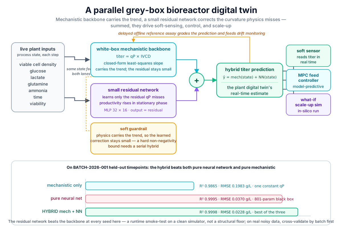 A parallel grey-box twin: a mechanistic backbone carries the trend, a small residual network corrects the curvature physics misses, and the summed prediction drives soft-sensing, control, and scale-up — with physics as the guardrail that keeps the trend physically anchored. (A hard non-negativity guarantee requires structurally embedding the ODEs, as in a serial hybrid or the model-predictive twin; this parallel residual form gets a softer benefit — the physics carries the trend, so the learned correction stays small.)
Original diagram by the authors, created with AI assistance.
A parallel grey-box twin: a mechanistic backbone carries the trend, a small residual network corrects the curvature physics misses, and the summed prediction drives soft-sensing, control, and scale-up — with physics as the guardrail that keeps the trend physically anchored. (A hard non-negativity guarantee requires structurally embedding the ODEs, as in a serial hybrid or the model-predictive twin; this parallel residual form gets a softer benefit — the physics carries the trend, so the learned correction stays small.)
Original diagram by the authors, created with AI assistance.
Here is the heart of the model, from examples/platform/ml/hybrid_model.py — the mechanistic fit, the residual network, and the pure-NN baseline it is measured against:
# examples/platform/ml/hybrid_model.py  (excerpt)
FEATS = ["Xv_e6_per_mL", "glucose_g_L", "lactate_g_L",
         "glutamine_mM", "ammonia_mM", "t_day", "viability_pct"]

def ivcd(df):                       # cumulative integral of viable cell density
    t  = df["t_day"].to_numpy()
    xv = df["Xv_e6_per_mL"].to_numpy()
    dt = np.diff(t, prepend=t[0])
    return np.cumsum(xv * dt)

def fit_qp(iv, y, idx):             # least-squares specific productivity (slope through origin)
    return float(np.sum(iv[idx] * y[idx]) / np.sum(iv[idx] ** 2))

def train_hybrid(test_size=0.3, seed=2026):
    df = load_state()              # fedbatch_state.parquet, minute -> hourly (336 rows)
    y  = df["titer_g_L"].to_numpy()
    iv = ivcd(df)
    X  = df[FEATS].to_numpy()       # Xv, glucose, lactate, glutamine, ammonia, t_day, viability
    tr, te = train_test_split(np.arange(len(df)), test_size=test_size, random_state=seed)

    qp   = fit_qp(iv, y, tr)        # the physics: one number, fit on TRAIN only
    mech = qp * iv

    resid  = y - mech               # the network learns ONLY what the physics misses
    scaler = StandardScaler().fit(X[tr])   # scaler fit on TRAIN only — no leakage
    nn = MLPRegressor(hidden_layer_sizes=(32, 16), max_iter=5000, alpha=1e-3, random_state=seed)
    nn.fit(scaler.transform(X[tr]), resid[tr])
    hybrid = mech + nn.predict(scaler.transform(X))

    nn_pure = MLPRegressor(hidden_layer_sizes=(32, 16), max_iter=5000, alpha=1e-3, random_state=seed)
    nn_pure.fit(scaler.transform(X[tr]), y[tr])   # pure black box: learns titer from scratch
    pure = nn_pure.predict(scaler.transform(X))
    # ... score mech / hybrid / pure on the held-out test rows, assert hybrid <= mech ...
Running it prints (verbatim from this dataset and seed):
Hybrid titer model on BATCH-2026-001 state (235 train / 101 test, qP=0.04049 g per 1e6 cell-day/mL):
  mechanistic only  R2=0.9865  RMSE=0.1983 g/L
  pure NN           R2=0.9995  RMSE=0.0370 g/L  (801 params)
  HYBRID (mech+NN)  R2=0.9998  RMSE=0.0228 g/L
ASSERT ok: the residual network lowers RMSE below the mechanistic backbone.
Read those three lines as the chapter's argument in numbers. The physics alone — a single constant qP = 0.04049 — already reaches R² = 0.9865 on held-out timepoints (R², the coefficient of determination, is the fraction of the variation in titer the model explains: 1.0 is perfect, 0 is no better than guessing the mean, so 0.9865 is already excellent), because IVCD genuinely drives titer; one fitted number gets you a root-mean-square error (RMSE — the typical size of the prediction's miss, in the same g/L units as titer, where smaller is better) of about 0.2 g/L. The pure network does better here (R² = 0.9995, RMSE 0.0370 g/L) but only because the simulator's state is almost perfectly informative; it spends its 801 parameters learning titer from scratch — the same 801-parameter network the hybrid uses, but pointed at a far harder target, which on real, noisy data with a few dozen real points it could rarely fit without overfitting. The hybrid posts the best error of the three (R² = 0.9998, RMSE 0.0228 g/L) using a network that only had to learn a small residual on top of the physics. The asserted check — the residual network beats the mechanistic backbone on the held-out split — passes at every seed here because the simulator's state is almost noiselessly informative, so a well-regularized residual is nearly free of risk. Read it as a runtime smoke-test, not a structural law: on real, noisy, few-dozen-point data an under-regularized residual network can overfit and lose to the backbone on a genuinely new run. That is exactly why the deployment version must be cross-validated by batch (above) before you trust the gap — the physics gives you a strong baseline to beat, not an automatic guarantee that the network will beat it.
Anatomy of one hybrid prediction
A digital twin does not emit a bare number; like every artifact in this series, a hybrid prediction is a structured record, and its value is in what travels alongside the estimate. When the twin fires for one timepoint of BATCH-2026-001, it produces a record whose fields encode the whole hybrid story — the physics contribution, the learned correction, the inputs, and the slow reference that will eventually grade it.
 One hybrid prediction, fully unpacked: the input state, the two-part decomposition into a mechanistic contribution and a learned residual, the summed estimate with its uncertainty, the delayed reference that grades it, and the provenance — fitted qP, architecture, seed, dataset hash — that makes it a governed record rather than a console line.
Original diagram by the authors, created with AI assistance.
One hybrid prediction, fully unpacked: the input state, the two-part decomposition into a mechanistic contribution and a learned residual, the summed estimate with its uncertainty, the delayed reference that grades it, and the provenance — fitted qP, architecture, seed, dataset hash — that makes it a governed record rather than a console line.
Original diagram by the authors, created with AI assistance.
Walk the record field by field, because each field is there for a reason a regulator would recognize:
- Identity header — the model name and version (
hybrid_titer_v1), the structure tag (parallel grey-box), the bound asset (BATCH-2026-001), and the timestamp the prediction is for. Version and structure are not cosmetic: under change control a prediction is only interpretable if you can name exactly which frozen model produced it. - Input block — the seven process-state features the network actually saw at that timepoint: viable cell density, glucose, lactate, glutamine, ammonia, time in days, viability. Logging the inputs verbatim is what lets you later re-run the prediction and prove it deterministic.
- Decomposition block — the core of the card and the thing no black box can offer. Two rows: the mechanistic contribution (
qPtimes IVCD, the physics's answer) in cyan, and the residual correction (the network's added term) in violet. They sum to the core value: the hybrid titer estimate in g/L, in green, paired with a model-uncertainty band. (The example network emits a point estimate; the uncertainty band in a deployed twin would come from a batch-resampled ensemble of residual networks or, more rigorously, split-conformal intervals calibrated on left-out batches — distribution-free coverage that respects the same leak-free batch-grouped split discipline the chapter mandates.) The split is the interpretability dividend made literal. - Reconciliation block — the delayed offline reference titer from the slow at-line assay, the residual between the twin's estimate and that reference once it lands, and an input-quality status flag that fires when a feature is out of range or stale. This is the block that grades the twin after the fact and feeds drift monitoring.
- Provenance footer — the dataset hash of the training data, the fitted
qPconstant, the network architecture (32 by 16), the random seed (2026), and the train/test split. Together these make the record reproducible to the bit and the model auditable: anyone can re-deriveqPand the split from the hash and confirm the number. A final note records the soft physics guardrail: the physics carries the trend, so the learned correction stays small — a plausibility benefit, not a hard non-negativity guarantee (that would require structurally embedding the ODEs, as in a serial hybrid or the model-predictive twin).
The record's most important property is that it is decomposable. A black-box prediction is a single opaque number; a hybrid prediction can always be split into "what the physics said" and "what the network added," and that split is exactly what a reviewer, an investigator, or a regulator wants. If the network's residual correction is small relative to the mechanistic term, the prediction is mostly trusted physics and is easy to defend. If the residual correction is large, that is a flag: the network is doing most of the work, the physics is being overruled, and the prediction has wandered into a regime the mechanistic model does not cover — precisely where you should distrust it. The ratio of the residual term to the mechanistic term is therefore a cheap, continuous trust gauge you get for free from the decomposition. This interpretability is a governance advantage no pure black box offers, and it is why hybrid models slot more comfortably into model-validation and QbD frameworks than their black-box cousins [1][6]. With the prediction record in hand, the rest of the chapter follows it outward — into the controller it can drive, the downstream twins it sits beside, and the ladder of scope it climbs.
What the record's fields refer to: the ontology under the twin
The fields above are named in prose, but a governed record needs them named in a vocabulary — otherwise "viable cell density" is a fragile column header that a CSV reshuffle or a vendor rename can silently break. The fix is to bind each field to a stable concept in a shared ontology (a machine-readable model of what the things in a domain are and how they relate; an IRI is the global identifier — an Internationalized Resource Identifier, the web-address-style name — that pins one concept). Pull the twin's glucose feature by its ontology IRI rather than by the string glucose_g_L, and a renamed column no longer breaks the model; the identifiers-and-units discipline also carries the unit (g/L) and the assay method with the value, so the network can never silently train on millimolar glucose mislabelled as grams per litre. This is the FAIR payoff (data that is Findable, Accessible, Interoperable, Reusable) made concrete for a model: a semantically grounded feature — one identified by its meaning, not its position — is the difference between a pipeline that survives a schema change and one that fails on the next campaign.
The same ontology types the bound asset in a way the bias-variance argument quietly depends on. The mAb campaign's domain model puts a measurement and the run it came from in different top-level categories — a measured titer is a continuant (a thing that persists, that has a value at a time) while the production run is an occurrent (a process that unfolds over time) — the BFO continuant/occurrent cut that keeps a reading distinct from the event that produced it. That distinction is exactly what tells the leave-whole-runs-out splitter which rows belong to the same run: the cross-validation grouping key is not a guessed column but the typed lineage edge. In the campaign's graph every artifact records what it bp:derivedFrom — the drug-substance lot from the bioreactor batch, the measurement from the run — and that PROV-O-style lineage chain (the W3C provenance vocabulary, prov:wasDerivedFrom, for who/what a record came from) is the same edge a leave-one-batch-out cross-validation groups on. The provenance footer's dataset hash and seed make a single prediction reproducible; the lineage graph makes the training set honest — it is what lets you prove no two timepoints of one run landed on opposite sides of the split.
That graph is also the schema a retrieval-grounded LLM stands on. When an investigator asks a natural-language assistant "what was this titer prediction derived from," a GraphRAG system answers by traversing the bp:derivedFrom edges — model version, training-dataset hash, the batch, the cell bank — rather than guessing from loose text, so the answer is grounded in the same provenance the record already carries. The ontology is what makes the graph mean what it claims; without it, "derived from" is a word the prose made up rather than a checkable edge.
Guaranteeing the training data is complete and in-range
A grey-box twin is only as trustworthy as the table it was fit on, and the data-governance question — is every required field present, in its declared unit, on a synchronized clock? — is upstream of every metric in this chapter. The training table is a slice of the plant's data shadow: time-series state from the historian, offline assay results from the LIMS, and batch context aligned to the ISA-95 equipment and material hierarchy (the manufacturing-systems standard whose Level 2/3 split names which signal belongs to which unit) and carried on standards like OPC UA off the floor and B2MML for the batch record. The hard part is rarely the model; it is reconciling a one-per-minute sensor stream with a once-a-day titer assay onto one timeline without smearing a stale value forward — exactly the timestamp-synchronization and missing-data rules the data-governance layer is there to enforce.
The clean way to make those rules executable is to reuse the release gate's own validation machinery. SHACL (the Shapes Constraint Language — a W3C standard for writing shapes, the rules a graph of data must satisfy) is how the release gate already checks that a lot's CQA panel is complete and in-range before the batch ships; the same shape, pointed at the model's input vector, guarantees the training and inference data are complete and in-range before the twin is allowed to fire. The input-quality status flag in the reconciliation block is precisely this check at inference time — a SHACL shape that trips when a feature is out of range or stale — so the discipline that gates a batch for a patient and the discipline that gates a row for a model are the same closed-world completeness check, written once. Validating the training set against the release-gate shape is the FAIR-and-governed answer to "garbage in, garbage out": a model fed only data that passed the same shape its product must pass is a model whose inputs you can defend to the same inspector.
The twin driving control: advisory model-predictive feeding
A digital twin is most valuable when it does more than watch — when its forward simulation actually shapes the next move. The hero diagram lists a model-predictive feed controller as one of the twin's three downstream uses, and the suite now makes that concrete with a runnable, advisory controller: examples/platform/ml/mpc_loop.py. It uses the mechanistic digital twin as its internal predictor — the same kind of physics backbone the hybrid carries — and asks it one question every control step: of all the feed moves I could make now, which best holds the process where I want it over the next few hours?
The general theory is receding-horizon (model-predictive) control, and it is worth stating faithfully because it is the same recipe whether the plant is a bioreactor or a refinery. At each control step the controller does four things. First, it reads the current state — here a noisy soft-sensor glucose estimate (a soft sensor is a model that infers a hard-to-measure quantity from easy-to-measure ones, in place of a physical probe), not a perfect measurement, exactly as the production-bioreactor soft sensor would feed it. Second, for each candidate feed move it rolls the twin forward a short horizon and scores the predicted trajectory against the setpoint, penalizing overshoot so the controller does not lurch. Third, it commits only the first move of the best-scoring plan — not the whole plan — and applies it. Fourth, at the next step it re-plans from scratch on a fresh (again noisy) measurement, so each decision is anchored to reality rather than to a stale forecast. That "plan a horizon, apply one step, re-measure, re-plan" loop is what makes the scheme robust to the twin being imperfect: errors are corrected every step instead of compounding over a fixed open-loop schedule. In our example the controller holds a 4.0 g/L glucose setpoint and acts every 12 h, proposing the feed bolus (a discrete shot of feed added at once, as opposed to a continuous trickle) that best tracks it, measured against an open-loop baseline that just delivers fixed boluses on a timer.
Running it prints (verbatim from this dataset and seed):
advisory soft-sensor MPC of glucose feed (setpoint = 4.0 g/L; control every 12 h)
  open-loop (fixed boluses)   : glucose tracking RMSE = 3.37 g/L, final titer = 5.77 g/L
  closed-loop (MPC, advisory) : glucose tracking RMSE = 1.09 g/L, final titer = 4.01 g/L
  note: the controller PROPOSES; in GMP a human / qualified automation with a safe fallback retains authority.
Read the two lines as a controlled comparison. The advisory loop holds glucose far closer to the 4.0 g/L setpoint than open-loop fixed boluses — a glucose-tracking RMSE of 1.09 g/L against 3.37 g/L, roughly a third of the open-loop error — while keeping the final titer healthy at 4.01 g/L (the open-loop run drifts to a higher 5.77 g/L precisely because it over-feeds against no setpoint). The controller earns the improvement by closing the loop: it sees where the soft sensor says glucose actually is and corrects, where the fixed schedule cannot.
One caveat the output does not print: here the controller's internal twin shares its kinetics verbatim with the simulated plant, so this run isolates the value of closing the loop under a perfect internal model — the 1.09-versus-3.37 g/L improvement is partly a gift of zero model-plant mismatch. In reality the twin is always somewhat wrong about the plant; the receding-horizon re-plan (apply one move, re-measure, re-plan) is exactly what keeps that mismatch from compounding, but a deployment must demonstrate robustness to it — which this clean demo deliberately does not stress-test.
The crucial qualifier is the one the output prints in plain language: the controller proposes. It does not act unattended. In GMP a human, or a qualified automation layer with a safe fallback, retains authority over the move that actually reaches the pump — which keeps this squarely inside the book's thesis that ML monitors and infers rather than autonomously decides, and inside the maturity framing of this chapter. A closed-loop twin steering a feed by itself is exactly the autonomous control that, as the maturity ladder and draft Annex 22 both make clear, is not how GMP runs today. So mpc_loop.py is a (pilot)-grade advisory demonstration of the digital twin steering a process, not a sketch of an autonomous GMP controller. It is the same line the whole-process and plant-twin rungs draw, brought down to one unit operation you can run.
Downstream: the chromatography twin leans mechanistic
Upstream twins are usually grey-box because cell physiology resists clean equations. Downstream, the balance tips the other way. Chromatography — the workhorse purification step that separates molecules by pumping the mixture through a column packed with porous beads, so different species travel at different speeds and emerge at different times (see the capture-chromatography chapter) — is governed by transport physics we understand well: the general rate model for mass transport through a packed bed (convection and axial dispersion — how the moving liquid carries and smears the band along the column; film transfer to the bead and pore diffusion inside it — how molecules cross into and through each porous bead), plus an adsorption isotherm — the curve relating how much protein sticks to the bead surface to how much is still dissolved in the liquid — such as steric mass action (SMA) for ion exchange (a separation that sorts molecules by electric charge, the bead surface carrying fixed charges that hold oppositely charged proteins), which models a bound protein as displacing counter-ions (the small mobile salt ions that were balancing the bead's surface charge) equal to its characteristic charge and sterically shielding further bound salt ions from exchange — the shielding being the "steric" in steric mass action. Given those equations and a handful of calibrated parameters — bed porosity, dispersion, the SMA characteristic charge and equilibrium constant — you can integrate the coupled PDEs (partial differential equations — the same rate-of-change idea as an ODE, but across space as well as time, because a column has position along its length) and simulate an elution chromatogram, predicting where the product peak and the impurities will come off the column under a given gradient. That is a mechanistic digital twin, and it is the most mature deployed computational technique in all of downstream processing — and it is mechanistic, not ML [7][8].
The production-grade incumbent is Cytiva GoSilico (acquired by Cytiva in 2021), whose ChromX/DSPX engine fits general-rate-plus-SMA models and is used in routine CMC process development (production) to replace racks of bench columns with in-silico runs — fitting model parameters from a small set of calibration gradients, then predicting unseen conditions. A peer-reviewed case from Hahn and colleagues built a mechanistic model of a pH-controlled mixed-mode polishing step from only six experiments and used in-silico optimization to improve the separation over the historical set point; a Sanofi team built a mechanistic hydrophobic-interaction model for vaccine-antigen purification [8][9]. The open-source counterpart is CADET, the same general-rate physics in a GPL-licensed solver, which makes the mechanistic approach reproducible without a vendor license. Where does ML enter? Only at the edges the physics does not reach: predicting the few hard-to-measure isotherm parameters from molecular descriptors when calibration data is thin, surrogate-modeling thousands of in-silico runs so an optimizer can search the design space quickly, or correcting for resin aging that the clean model ignores. A peer-reviewed (pilot) case from GenSci wrapped a mechanistic equilibrium-dispersive-plus-SMA model of a commercial PEGylated-protein AEX step with an ML correlation screen over 400-plus commercial lots, then ran tens of thousands of in-silico optimizations — though its yield and impurity-reduction headlines are self-reported by the authoring manufacturer on a single product and not independently reproduced [10]. The pattern is the mirror image of upstream: downstream, the physics is so strong that ML is the minority partner, and the capture and polishing chapters showed this thread step by step.
Up the ladder: unit twin, process twin, plant twin
A single grey-box bioreactor model is a unit-operation twin. The aspiration that excites the industry is bigger: chain the unit twins so a change upstream propagates through capture, viral filtration, polishing, and UF/DF (ultrafiltration/diafiltration — the final concentrate-and-buffer-exchange step), and you can ask "if I shift the feed strategy in the bioreactor, what happens to the host-cell-protein load — the residual protein from the producing cells themselves, an impurity the purification train must clear — on my polishing column?" That is a whole-process twin. Wider still is the plant twin — process plus utilities, scheduling, and equipment health — the lights-out factory of the keynote slides.
It is essential to be honest about where on this ladder reality actually sits, because the maturity drops fast with each rung:
- Unit-operation grey-box models are (production) to mature (pilot): deployed for soft-sensing, used routinely in development, and the strongest rung of the ladder. Grey-box CHO/mAb bioreactor models and mechanistic chromatography twins are real and in use [1][7].
- Whole-process twins are (pilot): demonstrated end to end in academic and consortium settings — an integrated continuous downstream twin spanning the standard purification chain — multicolumn Protein A capture, viral inactivation, and dual ion-exchange polishing — with online HPLC (a fast at-line analyzer reading product quality during the run) driving real-time pooling decisions (which fractions coming off the column to keep versus divert) is one published example [11] — but not running closed-loop across a commercial GMP train.
- Plant twins are (pilot) at best and largely aspirational. Siemens markets gPROMS-based whole-process and FormulatedProducts twins, and vendors demonstrate end-to-end bioprocess twins, but a fully closed-loop, whole-plant GMP twin that autonomously controls product quality does not exist in commercial production [12][13]. The ISPE Pharma 4.0 surveys keep landing on the same shape: AI/ML has the most pilots and the fewest scaled implementations, and what is in production clusters in monitoring, predictive maintenance, and vision — not autonomous control of CQAs.
A second honesty: there is no FDA or EMA guidance dedicated to digital twins. BioPhorum has published definitional whitepapers precisely because the lack of a shared definition slows regulatory acceptance — when "digital twin" can mean anything from a calibrated soft sensor to a fantasy autonomous factory, neither industry nor regulators can pin down what is being claimed [12][13].
The vendor landscape, attributed correctly
The twin market is small, consolidating, and routinely misattributed — so the corrections matter. Read each entry with two tags in mind: who owns it, and how mature the claimed capability is.
- DataHow (DataHowLab, SpectraHow) is the pure-play hybrid-modeling vendor: a grey-box engine plus transfer learning, with the peer-reviewed BMS case as its strongest evidence — maturity (pilot), process development. It is an independent ETH Zurich spin-off — its Series A was led by Momenta with Rockwell Automation and Zurich Kantonal Bank, and it announced an Eppendorf collaboration in December 2024 — and it is emphatically not owned by Sartorius [4].
- Insilico Biotechnology builds hybrid twins that pair a genome-scale metabolic model (a reconstruction of essentially all the cell's known metabolic reactions, used to predict consumption and production rates) with an ANN (artificial neural network) for soft-sensing and MPC — maturity (production/pilot), though full genome-scale models are rarely run directly inside a real-time twin (they are large and slow, so a reduced surrogate usually stands in). It was acquired by Yokogawa in November 2021 — not by Cytiva [14].
- Cytiva (Danaher) owns GoSilico for mechanistic chromatography modeling — mechanistic, not ML, maturity (production) in development — and markets a Bioreactor Scaler; its time- and yield-savings figures are vendor-self-reported [7].
- Sartorius/Umetrics wraps MVDA (multivariate data analysis — the workhorse statistical toolkit, e.g. PCA and PLS, for finding structure across many correlated process variables at once; its products here are SIMCA, MODDE, SIMCA-online) into a "Digital Twin AI Ecosystem" with Biobrain; the MVDA core is the production market standard, but the autonomous/self-optimizing layer is vendor-positioning and (pilot) [15].
- Siemens offers gPROMS-based whole-process and FormulatedProducts twins on top of its PCS 7/neo and SIPAT backbone — strong in chemical-engineering simulation, (pilot) for biopharma end-to-end [12].
The single-company headline numbers that circulate — WuXi's PatroLab "40-plus attributes, production-ready" Raman twin, Samsung's Plant 5 hybrid MPC — are press-release-only or vendor-self-reported and should never be cited as established fact; the companies' own executives concede much of the work is still manual.
The unsolved part: keeping the twin honest as the process moves
A digital twin's whole promise is that it stays faithful to the asset it mirrors. The unsolved problem is that the asset keeps moving and the twin does not know it. A grey-box bioreactor model fit on this season's cell bank, this raw-material lot, and this scale will drift the moment any of those change — and the same sparse-reference regime that makes the model necessary makes its drift invisible. The hybrid structure helps but does not solve it: the physics keeps the prediction plausible, so a drifting hybrid still returns a sensible-looking titer, which can be more dangerous than a black box that returns obvious nonsense. The guardrail that protects you from absurdity is the same guardrail that hides the slow lie.
The decomposability of the record is the best handle we have, and it is more than a metaphor. The reconciliation block gives two measurable drift signals. The first is the residual-versus-reference series: each time the slow offline assay lands, the twin's error is logged, and a creeping bias in that series — predictions drifting consistently high or low — is drift you can see before any single point looks wrong. The second is the decomposition ratio: when the network's residual contribution grows as a fraction of the mechanistic term over a campaign, the twin is leaning harder and harder on the learned correction to match reality, which is drift visible before the offline assays even accumulate, because it shows up in the model's own internals. Turning "the residual is getting large" into a validated alarm with a defined threshold, under change control, is exactly the MLOps and validation problem the next chapter takes head-on.
And the deepest open question is structural: a twin that retrains itself to track the moving process is, under GMP, a model that changes its own behavior — which the regulators have decided to constrain rather than embrace. Draft Annex 22 draws a sharp line, covering only static (locked) models whose parameters are fixed during use and explicitly excluding generative and continuously-adaptive AI from critical GMP applications; GMP-critical AI must be a locked model governed by a predetermined change control plan, with the US FDA's predetermined change control plan (PCCP) guidance the parallel concept on the device side. A self-updating twin is precisely what draft Annex 22 says you may not run unattended on a quality-critical decision. The honest state of the art is therefore a twin that is re-validated on a schedule — re-fit offline, re-qualified, re-locked under change control — not one that quietly keeps learning [16][17].
What this chapter adds to the model suite
This chapter consolidates the hybrid thread that ran through the upstream chapters into one named, runnable module:
examples/platform/ml/hybrid_model.py— the parallel grey-box titer twin forBATCH-2026-001: a mechanistic IVCD-times-qPbackbone, anMLPRegressorresidual network over the process state, and a pure-NN baseline for comparison, all overexamples/datasets/fedbatch_state.parquet. Its asserted check — the residual network lowers RMSE below the mechanistic backbone — passes at every seed on this clean simulator, encoded as a runtime smoke-test; on real noisy data it is an empirical tendency to verify by batch-grouped cross-validation, not a structural law. It is the consolidation point for the production-bioreactor soft sensor (soft_sensor_pls.py,soft_sensor_deep.py), and the upstream counterpart to the mechanistic chromatography model (chromatography.py) — together they are the book's two-sided answer to the small-data problem: grey-box where physiology is messy, mechanistic-plus-ML where transport physics is strong.examples/platform/ml/mpc_loop.py— an advisory receding-horizon controller that puts the digital twin in the loop: it reads a noisy soft-sensor glucose estimate, rolls the mechanistic twin forward a short horizon every 12 h, and proposes the feed bolus that best holds a 4.0 g/L setpoint, scored against open-loop fixed boluses (glucose-tracking RMSE 1.09 vs 3.37 g/L). The controller proposes; a human or qualified automation with a safe fallback retains authority — a (pilot)-grade demonstration of a twin steering a process, not autonomous GMP control.
Why it matters
Hybrid modeling is the reason this book is not a catalog of clever demos that never ship. Every chapter's model lives or dies on the same constraint — too few batches, too costly to gather more — and the move that lets a model survive that constraint is to stop asking the data to learn what physics already knows. The hybrid is not a compromise between mechanistic and ML; in the small-data regime that defines biomanufacturing, it routinely beats both [1][2]. It is also the form of ML that fits governance best: a prediction you can split into trusted physics plus a visible correction is a prediction you can defend to a regulator, monitor for drift, and bound with a guardrail. Get hybrid modeling right and the soft sensors, controllers, and scale-up tools of the previous twenty chapters become deployable; insist on pure black boxes and they stay in the lab.
In the real world
The production-grade reality is narrower and more useful than the digital-twin headlines suggest. Grey-box bioreactor models are deployed for soft-sensing and used routinely in development; mechanistic chromatography twins (Cytiva GoSilico, open-source CADET) are the most mature deployed computational technique downstream and are mechanistic, not ML [7][8]. The flagship hybrid case — DataHow with Bristol Myers Squibb — is peer-reviewed (pilot) at process-development scale, reporting roughly 33 percent better accuracy with about half the data; the larger vendor figures are self-reported [4]. Insilico's genome-scale-plus-ANN twins under Yokogawa are (production/pilot), though full genome-scale models are rarely used directly in real-time twins [14]. Whole-process and plant twins from Siemens and others are (pilot) or aspirational, with no fully closed-loop GMP plant twin in production [12][13]. The frontier sits at self-driving development: a (research) DataHow/Sartorius/Merck study ran 27-day autonomous perfusion cultivations (a continuous-feed culture mode that constantly adds fresh medium and removes spent, sustaining cells far longer than a fed-batch) on a 24-parallel mini-bioreactor platform using a Bayesian experimental-design algorithm plus a cognitive digital twin — "cognitive" here meaning the twin not only mirrors the process but actively chooses the next experiment to run, closing the design-decide-execute loop — and even its authors stress the gap between robotic capability and true device autonomy [18]. The pattern is consistent across the whole landscape: hybrid modeling is real and winning; the autonomous twin is not here yet.
Key terms
- Hybrid (grey-box / semi-parametric) model — a model combining a mechanistic (first-principles) backbone with a data-driven component that covers what the physics cannot write down.
- Mechanistic / white-box model — a model built entirely from physics and chemistry equations (mass balances, kinetics, transport), with no learned parameters fit to outcome data.
- Serial vs parallel hybrid — serial: the network feeds a quantity (e.g. a kinetic rate) into the mechanistic equations, which are then integrated; parallel: the network learns the residual the mechanistic model gets wrong, added to the physics prediction.
- Physics-informed neural network (PINN) — a network that carries the governing equations as a soft penalty in its loss (a weighted equation-residual term over collocation points), rather than structurally embedding them; weaker than a true hybrid under extrapolation.
- Bias-variance trade-off — the statistical reason physics helps: embedding known equations shrinks the hypothesis space, cutting variance so a few batches suffice.
- IVCD (integral of viable cell density) — the running time-integral of viable cells; with a specific productivity
qPit is the classic mechanistic predictor of accumulated titer. - Specific productivity (
qP) — antibody secreted per cell per unit time; the single constant the mechanistic backbone fits by least squares through the origin. - Digital twin — a model (here, hybrid) wired to live plant data so it tracks a real asset in real time, used for soft-sensing, control, and what-if simulation.
- Unit / process / plant twin — the ladder of scope: one unit operation, a chained process train, or a whole facility including utilities and scheduling — with maturity dropping fast up the rungs.
- General rate model + steric mass action — the transport-plus-adsorption physics behind mechanistic chromatography twins.
- CPP / CQA — critical process parameter (a controllable input like feed rate, temperature, or pH) versus critical quality attribute (a measured product property, like titer or aggregation, that must stay in spec for release).
- GMP (Good Manufacturing Practice) — the legally binding quality framework medicines must be manufactured under; draft EU/PIC/S Annex 22 is its emerging AI annex, co-developed with the international PIC/S inspectorate.
- Locked model / predetermined change control plan (PCCP) — a model frozen for use, with any future change governed by a pre-approved plan; the regulatory posture draft Annex 22 requires of GMP-critical AI, excluding self-adapting models.
- Ontology / IRI — a machine-readable model of what a domain's things are and how they relate, each concept pinned by a global identifier (IRI); pulling a feature by its IRI rather than a column name is what keeps a model from breaking on a schema change.
- Semantically grounded feature — a model input identified by its ontology concept (and so carrying its unit and assay method), not by its fragile position or column string; the FAIR, schema-change-resistant alternative.
- PROV-O lineage /
bp:derivedFrom— the provenance edge recording what a record came from (lot from batch, measurement from run); the same typed link that supplies the grouping key for leave-one-batch-out cross-validation. - SHACL shape — a reusable rule a graph of data must satisfy; the release gate's own completeness-and-range check, pointed at the model's input vector to guarantee training and inference data are complete and in-range.
Where this leads
A hybrid twin is only as trustworthy as the discipline that keeps it current. The next chapter, MLOps and Lifecycle: Drift, Retraining, and the Validation Paradox, confronts the problem this one ended on: a model decays the moment the living process moves, yet GMP demands a locked, validated model — so how do you retrain a thing that is not allowed to change itself? It builds the monitoring, drift-detection, and change-control machinery that turns a clever model into a deployable one, and resolves the validation paradox that hangs over every prediction in this book.