Manufacturing Operations: Predictive Maintenance, Yield, and Scheduling
📍 Where we are: Part VI · The Whole System — Chapter 23. The last chapter built the MLOps spine — drift, retraining, and the validation paradox — that keeps any single model honest after deployment. Now we pull back from the model to the plant: the equipment, the schedule, and the batch outcome that all those unit-operation models add up to.
Every chapter before this one looked down a microscope at one step — a soft sensor on one bioreactor, a hybrid model of one capture column, a vision system on one filling line. This chapter looks up, at the factory as a system: a hall full of vessels, skids, chillers, and air handlers that wear out; a calendar of batches competing for those vessels; and, at the end of each campaign, a release decision that is either a clean pass or an expensive failure. The machine learning that lives at this altitude is the least glamorous in the book and, not coincidentally, the most deployed. It rarely touches a critical quality attribute (CQA — a measurable property like purity or potency that defines whether the drug is fit to release) directly. It keeps a motor from seizing, flags a batch that is drifting toward an out-of-spec result (a measured value outside its registered specification limit — a batch that fails release), drafts the review of a clean record so a human only reads the exceptions, and packs more product into the same steel.
This is also where the running example finally pays a debt. Across five books we have followed BATCH-2026-001 and its siblings, and we have always known there was one out-of-spec sibling, BATCH-2026-004. In this chapter it stops being a footnote and becomes a target: the positive label a batch-failure model is trying to predict before the lab confirms it. The honest part of the story is that with six batches you cannot train such a model — and that constraint, not the algorithm, is the real subject.
A good factory manager does three boring, valuable things. They listen to the machines — a bearing that sounds slightly rough today will fail next month, so fix it on a planned Saturday, not in the middle of a batch. They watch each batch as it runs and develop a gut feel for "this one's going sideways" before the final test confirms it. And they pack the schedule so no expensive vessel sits idle. Plant-level machine learning is software that does exactly those three things — predict the breakdown, predict the bad batch, pack the calendar — from the data the plant already generates. None of it cures cancer; all of it keeps the lights on and the steel full.
What this chapter covers
We move up a level of abstraction, from the unit operation to the plant, and walk the four families of operations ML that actually run in industry:
- Predictive maintenance (PdM) — learning an equipment-health signal from vibration, current, and temperature so a failure is caught with lead time, framed as the unsupervised "departure from healthy" problem it usually is.
- Batch-failure / yield / deviation prediction — a batch-level supervised task (one row per batch, not per second), with
BATCH-2026-004's real host-cell-protein (HCP) excursion as the failure mode, and an honest reckoning with the six-batch data ceiling. - Right-first-time and review-by-exception — how ML rides on top of the Manufacturing Execution System (MES — the software that executes and records the batch recipe on the floor) execution layer (Körber PAS-X) to shrink the human review burden, and where the regulatory line forbids it from going further.
- Scheduling, capacity, supply-chain, and energy — the optimization and forecasting problems that are mostly not deep learning, and where the real money is.
Three runnable modules anchor the chapter, presented in reading order: examples/platform/ml/pdm.py (an illustrative predictive-maintenance signal), examples/platform/ml/batch_outcome.py (yield/failure prediction grounded in the real release table), and examples/platform/ml/integration_opcua.py (the interface contract a prediction must satisfy to cross into the control system — over OPC-UA, the open industrial communication protocol that puts a tagged value on a plant tag, into a historian, the time-series database that keeps the plant's tag history, and the MES).
Predictive maintenance: the plant's most reliable ML
Ask a manufacturing-systems engineer where machine learning has actually earned its keep on the shop floor, and the answer is rarely "the bioreactor." It is the equipment around the bioreactor. A bioreactor's agitation motor, a chromatography skid's feed pump, a centrifuge's drive, a chiller compressor, an HVAC supply fan — each is a rotating or reciprocating machine with a physical signature (vibration spectrum, motor current, bearing temperature, acoustic emission) that drifts slowly as a bearing spalls (its surface starts to flake) or a seal degrades, often weeks before the part actually fails [1]. The economic case is stark: an unplanned failure mid-batch can scrap a multi-week run worth far more than the part; a planned swap on a maintenance Saturday costs the part and an hour.
The thing that makes PdM tractable where CQA prediction is hard is the labels. A soft sensor (a model that infers a hard-to-measure quantity from cheap signals) needs the expensive offline reference — the lab measurement of the true value — to learn from. PdM mostly does not, because real catastrophic failures are too rare to train a supervised classifier on (a supervised model learns from examples that are each tagged with the right answer — here, "failed" or "healthy") — you may have one bearing failure per pump per several years. So the deployable formulation is almost always unsupervised (it learns the shape of the data with no answer labels at all): learn what "healthy" looks like from a baseline window of normal operation, then alarm when the live signal departs from that envelope. This is the same conceptual move as the golden-batch envelope and MSPC: build a model of normal, score novelty against it. The simplest version is a one-dimensional control chart on a vibration RMS (root-mean-square, the overall energy of the vibration signal); the richer versions score how far a multi-sensor reading is from the healthy cloud — for example a PCA/autoencoder reconstruction error (how badly a model trained on healthy data fails to rebuild the new reading), with an isolation forest or one-class SVM (two other detectors that simply carve out the region the healthy data occupies and flag anything outside it) as common alternatives — where that residual is the health score. Each of these is unpacked in the ladder below.
One bio-specific caveat keeps the scope honest: the departure-score story here is the universal rotating-equipment one, but in a biologics plant the failure that most often scraps a batch is a sterility or integrity loss — a single-use bag weld, a sterilizing-grade filter, or a clean-utility excursion — which a vibration z-score never sees. Those are watched by pre/post-use integrity tests and clean-utility (WFI — water for injection, the ultra-pure water the plant runs on — and clean steam) quality trending, a different monitoring discipline that sits beside, not inside, the rotating-asset PdM ladder.
Four ways to model "normal," ranked by what they need
The unsupervised PdM family is a ladder, and the rung you climb to is set by how many sensors you have and how early you need the warning, not by sophistication for its own sake.
- Univariate control chart. One scalar — a daily vibration RMS, a motor current — with the mean and standard deviation of a healthy window as the limits. The health score is the standardized departure (the live value minus the baseline mean, divided by the baseline standard deviation), alarmed at three sigma — three standard deviations from the healthy mean, the conventional alarm point because a healthy signal almost never strays that far by chance — exactly as in SPC (statistical process control, the classic control-chart discipline for spotting when a process leaves its normal range). Cheapest, most auditable, and the floor below which any richer method must prove it adds value.
- Multivariate PCA / Hotelling's T-squared. Stack several correlated channels (vibration, current, two bearing temperatures), fit a PCA — principal component analysis, which finds the few combined directions along which healthy data actually varies — on the healthy window, and monitor two statistics. The T-squared distance measures how far a reading sits along those normal directions (drift the model expected, just more of it); the squared prediction error, SPE or Q, measures how far it sits off them (a genuinely new pattern the healthy model never saw — "orthogonal" just means in a direction the model has no axis for). The SPE side is the one that catches a genuinely novel fault, and the per-variable SPE contribution tells you which sensor broke — the same diagnostic the MSPC module uses to point at HCP on
BATCH-2026-004. - Reconstruction error from an autoencoder. An autoencoder is a small neural network trained to squeeze a reading down to a few numbers and then rebuild it; trained only on healthy data, it rebuilds healthy readings well and unfamiliar ones badly. So when it runs on new data (at inference), the reconstruction residual — the gap between the input and the rebuilt version — is the health score. It captures nonlinear couplings a linear PCA misses, at the cost of more data to fit and a model that is harder to explain to an inspector.
- Isolation forest / one-class SVM. Pure novelty detectors that carve out the region the healthy data occupies and score anything outside it as an anomaly — the same isolation-forest pattern the viral-clearance module flags a fouled filtration run with and the serialization layer scores a short case with. Useful when "normal" is a strangely shaped cloud, but they give a score, not a calibrated probability, and no native diagnostic of which signal moved.
Each rung answers the same question — how far is today from healthy? — and differs only in how much structure it can represent and how much data and explanation that costs. In a GMP (Good Manufacturing Practice — the legally enforceable quality rules a regulated drug plant runs under) plant the explainability cost is real: a univariate chart and a PCA SPE-contribution plot survive an audit on their own arithmetic — an inspector can re-derive every number by hand — whereas an autoencoder residual needs the same intended-use scoping (a written statement of exactly what the model may and may not be used for), change control (every change formally reviewed and approved), and human disposition (a qualified person, not the model, making the final call) the MLOps chapter demands of any model whose internals an inspector cannot read off the page.
The departure score, concretely
The reliable, auditable PdM pattern is a z-distance from a healthy baseline. Take a daily vibration RMS for an agitation motor, fit the mean and standard deviation over a baseline window of known-good days, and express every later day as a number of standard deviations from that baseline. When that departure crosses an alarm threshold — three sigma is the natural choice, borrowing the SPC convention — you have an alarm, and crucially you have it with lead time before the hard failure. The lead time is the entire value: it converts an emergency into a scheduled task. (In a real program the relative departure score sits alongside an absolute benchmark — overall vibration velocity, in millimetres per second, graded against ISO 20816, the international standard that sorts machine vibration into "good / acceptable / unsatisfactory / unacceptable" severity classes — so an alarm is anchored to a physical severity scale as well as to drift from this machine's own healthy window; the 1.8 mm/s baseline used below is in the realistic "good" range for a small machine.)
The arithmetic is deliberately the univariate floor. The baseline window must come from known-good days — fit the mean and standard deviation only on the healthy stretch, never on the whole trace, or the wear you are trying to detect leaks into your own limits and the alarm never fires. Use the sample standard deviation (divide by the count minus one, ddof=1, rather than by the count), because on a small window dividing by the count slightly under-estimates the true spread; the minus-one correction removes that systematic lean (an unbiased estimate is one that is right on average rather than consistently too small) — and it matters when only twenty-one days set the threshold for the next month. The alarm is the first day the departure exceeds three sigma, and the lead time is the gap from that day to the eventual hard failure:
# examples/platform/ml/pdm.py
def health_score(signal: np.ndarray, baseline_days: int = 21) -> dict:
    """Unsupervised PdM: z-distance from the healthy baseline window."""
    base = signal[:baseline_days]
    mu, sd = base.mean(), base.std(ddof=1)
    z = (signal - mu) / sd                              # departure score
    alarm = 3.0                                         # 3-sigma, an SPC threshold
    crossed = np.argmax(z > alarm) if (z > alarm).any() else -1
    return {"baseline_mean": round(float(mu), 3),
            "baseline_sd": round(float(sd), 3),
            "alarm_threshold_sigma": alarm,
            "first_alarm_day": int(crossed),
            "max_z": round(float(z.max()), 2)}
The richer the feature, the earlier the warning. A raw vibration amplitude only spikes near the end; a spectral feature — energy at the bearing's characteristic defect frequency, or the kurtosis of the high-frequency band (kurtosis measures how "spiky" a signal is, and an early bearing fault shows up as sharp impacts long before the overall level rises) — moves much sooner, which is why production PdM platforms (AVEVA Predictive Analytics, Siemens Senseye, the equipment-analytics layer in Aizon and Rockwell) lean on frequency-domain features rather than a single scalar [1][2]. The method below is deliberately the scalar version, because it is the honest floor: if even a one-number z-score buys lead time, the spectral version buys more.
Remaining useful life versus anomaly: two different questions
PdM splits into two questions that the same z-score does not answer equally. The first is anomaly detection — is the machine departing from healthy now? — which the departure score answers directly and is what almost every deployed biopharma PdM system actually does. The second, harder question is remaining useful life (RUL) — how many days until failure? — which is a regression onto time-to-event (a model that predicts a number of days rather than a yes/no), and it needs run-to-failure histories — full records of machines tracked all the way to the moment they broke — that the plant rarely has. RUL is where the published research lives (degradation-trajectory models, particle filters, and recurrent and survival models — a family of methods for learning how long a process runs before an event — trained on engine and bearing run-to-failure benchmarks), but it is also where the data ceiling bites hardest: you cannot learn the shape of a degradation curve from machines that have failed once or never. So the deployable reality is the anomaly side — fire an alarm with lead time — and "remaining useful life" in practice is usually the crude but auditable extrapolation of the departure trend to its threshold, not a learned survival model. The same labels-are-scarce constraint that governs batch failure governs equipment failure, which is exactly why both deployable answers are unsupervised.
Batch-failure prediction: the OOS as a target
Predictive maintenance is about the equipment. The second family is about the product: can a model, partway through or at the end of a run, predict whether the batch will pass release — the final go/no-go decision that lets a batch be shipped, or rejects it as an out-of-spec (OOS) result, a value outside its registered specification limit? This is batch-failure prediction (and its continuous cousins, yield prediction and deviation prediction), and it is a genuinely different ML task from everything earlier in the book — because the unit of analysis is the batch, not the timepoint.
That distinction is the whole difficulty. A Raman soft sensor (a model fed a Raman spectrum — an optical fingerprint of what is dissolved in the broth, measured continuously) has thousands of training rows from a single batch, because it makes a fresh prediction every minute as that spectrum changes. A batch-failure model has one row per batch — a fixed-length vector of process-summary features (peak viable cell density, integral lactate, harvest turbidity, capture load, cumulative hours outside the temperature NOR) paired with one binary outcome, pass or fail. The number of rows is the number of batches you have ever run, and that is the binding constraint of the entire plant-level enterprise [3]. A commercial process at a single site might accumulate a few hundred batches over years; a clinical or new-product process has a handful. This is the small-data ceiling from Chapter 1, at its most severe, because here it is measured in batches rather than rows.
Featurizing a batch: from time series to one row
The modeling move that defines this family is featurization: collapsing each batch's multi-day, multi-sensor time series into one fixed-length vector. A batch is not a row — it is dozens of tag trajectories sampled every few seconds for two weeks — and the model needs every batch reduced to the same handful of numbers so that "one row per batch" is even well-defined. The six features in the example are each a deliberate summary statistic of a trajectory chosen to be physically meaningful, not a raw reading:
peak_VCD_e6_per_mL— the maximum of the viable-cell-density curve, an upstream growth summary.final_titer_g_L— the productivity endpoint.integral_lactate— lactate concentration integrated over time (an area under the curve, the metabolic-burden summary), the same trajectory-integral idea as the integral-VCD feature in the release-prediction module.harvest_turbidity_NTU— the turbidity (cloudiness, in nephelometric turbidity units, NTU) of the clarified pool downstream of the centrifuge and depth filter; clarification carry-over and the HCP-risk driver. The harvest chapter models the pre-clarification harvest-feed cloudiness (which runs far higher); clarification then drives it down to the under-5-NTU clarified target, and it is that residual carry-over the feature captures here. A well-clarified run sits low near that target; a poorly-clarified run drifts higher.protein_a_load_g_L— capture column loading.temp_excursion_h— cumulative hours outside the temperature normal operating range (NOR — the validated band the parameter is meant to stay within), an event-count over the run.
Peaks, endpoints, integrals, and excursion-counts are the four featurization idioms, and the choice of which to extract is the domain knowledge — it is where a process engineer, not the algorithm, encodes what about a batch could plausibly drive a failure. A model fed raw timepoints would have to relearn this from data it does not have; a model fed good summaries starts from physics.
In practice the feature vector is not built once at release but grows as the batch advances — peak VCD and integral lactate land at end of culture, turbidity at harvest, capture load after the column — so the model is re-scored at each milestone. This is the multiway / evolving-batch-monitoring idiom (Nomikos and MacGregor's batch PCA/PLS — "multiway" simply means the batch's full time-by-sensor grid is unfolded into one long feature row so the same PCA/PLS modelling applies to a whole batch as it progresses) that lets an end-of-capture warning still leave room to re-pool before an OOS locks in, and it is exactly the as-of phase framing the anatomy figure later pins. The same temporal logic refines the PdM side: above the static daily z-score the departure is usually smoothed with an EWMA or CUSUM (two classic running-average filters that react to a sustained shift but ignore a single noisy day) so one bad reading does not trip the alarm — trading a little lead time for far fewer false alarms — with matrix-profile and small recurrent detectors (pattern-matching and sequence-learning methods that spot an unusual stretch of signal) as the research-grade rung above that where run-rich histories exist [2]. The static z stays the deployable floor.
The running example: BATCH-2026-004
The campaign in this series carries exactly one out-of-spec sibling. Read straight from examples/datasets/hplc_results.csv, the failure is unambiguous: BATCH-2026-004 has a host-cell-protein result of 128.0 ng/mg against a specification ceiling of 100.0 ng/mg — the only OOS value in the entire 66-row release table; every other assay on every batch passes. The other five batches (BATCH-2026-001/002/003/005/006) are clean, with HCP values from 14.953 to 28.203 ng/mg, all comfortably inside spec. So the label a batch-failure model would learn is real and it is single-attribute: this batch failed on HCP, host-cell-protein carry-over, not on monomer purity (the fraction of product that is the correct single molecule rather than clumped aggregate), charge variants (slightly modified forms of the antibody that carry a different electrical charge), or any other CQA.
The mechanism matters for the features. Host-cell protein is a downstream-clearance attribute, and HCP that survives the capture and polishing steps traces back to two things the plant can summarize per batch: how much host-cell debris entered downstream (a turbid harvest carries more forward, set at harvest and clarification) and how the capture column was loaded and washed. Load is one lever among several — clearance across Protein A is governed at least as much by wash design, elution pH, and resin selectivity, and load drives HCP mainly when it pushes the column toward its dynamic binding capacity (the most product the resin can actually hold under flow) so that weakly-bound HCP co-elutes (comes off the column together with the product instead of being washed away). But the two summary features available to a batch-level model here are harvest turbidity and capture load, so a physics-shaped model should find those as the readable proxies for an HCP failure — not the upstream growth metrics that drive titer. A model that instead "predicts" the failure from, say, peak VCD would be learning a spurious correlation, and on six batches it absolutely could. This is the same diagnosis the MSPC module reaches from the other direction: when it flags BATCH-2026-004 with an SPE (the squared prediction error from the PCA monitor above) of 356.59 against a 4.95 alarm limit — far outside normal — fully 83% of that error traces to the HCP channel; multivariate monitoring and batch-failure prediction agree on which attribute and which mechanism, which is the cross-check that makes either credible.
Why six batches cannot train a classifier
Here is the honest core. With six batches and one failure, you cannot fit, validate, or trust a batch-failure classifier — full stop. One positive example is not a class; the standard test is to hold out part of the data as a fold the model never trains on and score it there, but with one failure a single held-out fold either contains the failure (and the train set has none) or it does not (and the test set has none). Any AUC (area under the ROC curve — a 0-to-1 summary of how well the scores rank failures above passes, 0.5 being a coin flip and 1.0 perfect) you report is an artifact. The lesson of this chapter is not "look, we built a batch-failure model"; it is "here is what the model would look like, here is the data you would need, and here is why the plant-level constraint is batches-not-rows." And the count overstates what you can actually use: across a product's life, comparability exercises (formal studies proving the product is unchanged after some manufacturing change), scale changes, resin and media lot changes, and method transfers (moving a process or assay to a new line or site) re-partition the population, so even a mature site's hundreds of batches are not one exchangeable distribution but several — the same non-stationarity that breaks transfer learning, arriving here as the reason the usable training set is smaller than the batch count suggests.
So the example module does two things side by side, and labels the boundary loudly. It reads the real outcomes from hplc_results.csv and batches.csv to state the ground truth (5 PASS, 1 OOS, the HCP excursion). Then it builds an illustrative synthetic cohort of a few hundred batches around the real process statistics — with failure driven by harvest turbidity into HCP carry-over, the real BATCH-2026-004 mechanism — purely to demonstrate the gradient-boosted classifier and its feature attribution. The model is real; the cohort it trains on is synthesised, and every number it prints is marked illustrative. That is the only intellectually honest way to show plant-level ML on a six-batch dataset.
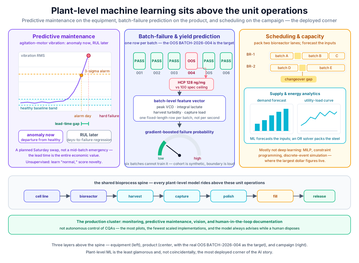 Plant-level learning sits above the unit operations: predictive maintenance on the equipment (left), batch-failure and yield prediction on the product (center, with the real OOS BATCH-2026-004 as the target), and scheduling, capacity, supply-chain, and energy analytics on the campaign (right) — the cluster where production ML actually lives.
Original diagram by the authors, created with AI assistance.
Plant-level learning sits above the unit operations: predictive maintenance on the equipment (left), batch-failure and yield prediction on the product (center, with the real OOS BATCH-2026-004 as the target), and scheduling, capacity, supply-chain, and energy analytics on the campaign (right) — the cluster where production ML actually lives.
Original diagram by the authors, created with AI assistance.
Building the two models
The chapter's two modules are pure NumPy/Pandas/scikit-learn over the committed datasets, so they run with no services. Start with the batch-outcome model. It reads the real release outcomes, then trains a gradient-boosted failure classifier on the illustrative cohort, cross-validated batch-out — scoring each batch only with models that never saw it, explained two paragraphs below — because that is the only honest small-data estimate:
# examples/platform/ml/batch_outcome.py
from sklearn.ensemble import GradientBoostingClassifier
from sklearn.metrics import roc_auc_score
from sklearn.model_selection import cross_val_predict

# Plant-level summary features a completed batch carries by harvest/release.
FEATURES = [
    "peak_VCD_e6_per_mL",    # upstream growth summary
    "final_titer_g_L",       # productivity summary
    "integral_lactate",      # metabolic-burden summary (lactate * time)
    "harvest_turbidity_NTU", # clarification carry-over -> HCP risk
    "protein_a_load_g_L",    # capture loading
    "temp_excursion_h",      # cumulative hours outside the temperature NOR
]

def real_release_outcomes() -> pd.DataFrame:
    """The ground truth: 6 batches, one OOS. Read straight from the datasets."""
    hplc = pd.read_csv(DATASETS / "hplc_results.csv")
    batches = pd.read_csv(DATASETS / "batches.csv")
    oos = hplc[hplc.result == "OOS"][["batch_id", "test", "value", "spec_high"]]
    return batches.merge(oos.rename(columns={"test": "failing_assay",
                                             "value": "failing_value"}),
                         on="batch_id", how="left")

def train_failure_model(df: pd.DataFrame) -> dict:
    """Gradient-boosted batch-failure classifier, batch-out cross-validated."""
    X, y = df[FEATURES].to_numpy(), df["failed_release"].to_numpy()
    clf = GradientBoostingClassifier(n_estimators=200, max_depth=2, random_state=2026)
    # 5-fold CV is the honest small-data estimate; never score on the train fold.
    proba = cross_val_predict(clf, X, y, cv=5, method="predict_proba")[:, 1]
    auc = roc_auc_score(y, proba)
    clf.fit(X, y)
    imp = dict(sorted(zip(FEATURES, clf.feature_importances_), key=lambda kv: -kv[1]))
    return {"n": len(df), "n_failed": int(y.sum()),
            "cv_auc": round(float(auc), 3), "top_driver": next(iter(imp)),
            "importances": {k: round(float(v), 3) for k, v in imp.items()}}
The algorithm choice is not incidental. A gradient-boosted classifier — a team (ensemble) of small decision trees added one at a time, where each new shallow tree is trained to correct the errors the trees before it still make (formally, to fit the gradient of the loss they left over) — is the right default for batch-level tabular data for three reasons that a neural network cannot match here. It handles a handful of heterogeneous features (a viable-cell density, a turbidity, an hour-count) on different scales with no preprocessing; it captures the threshold-and-interaction structure of real failures (HCP fails when turbidity is high and load is high) through tree splits rather than needing the interaction hand-coded; and with shallow trees (max_depth=2, so each tree sees at most a two-way interaction) it resists overfitting the way a deep network on a few hundred rows would not. The random_state=2026 makes the boosting reproducible, which the MLOps chapter insists on for any model whose number lands in a record.
The validation choice is where the honesty lives. cross_val_predict with five folds produces an out-of-fold probability for every batch — each batch is scored by a model that never saw it — and the AUC is computed on those held-out predictions, never on the training fold. On real batches this is batch-out cross-validation: the only defensible small-data estimate, because scoring a batch with a model that trained on it would report the memorization, not the generalization. With one real failure the procedure still cannot save you — a five-fold split of six batches is a parody — which is exactly why the cohort is synthetic and the boundary is loud. The feature importances come from the fitted model's mean impurity decrease per feature, summing to one — "impurity" being how mixed the pass/fail labels are in a tree branch, so a feature that splits them cleanly looks important — but this impurity (Gini) importance is biased (it under-credits yes/no features and over-credits continuous ones with many distinct values, simply because they offer the trees more places to split), so it is only the first-pass read; the actionable attribution an investigator should trust is the permutation importance (or SHAP) introduced below.
Running python ml/batch_outcome.py prints the real ground truth, then puts the illustrative model through the same credibility review a deployable model would face — not just a headline AUROC but its uncertainty, its calibration, and a model-agnostic attribution:
REAL release outcomes (6 batches):
  5 PASS, 1 OOS
  OOS batch = BATCH-2026-004: HCP_ng_per_mg = 128.0 (spec <= 100.0)

batch-failure classifier (ILLUSTRATIVE cohort, n=240, 39 failed, rate=0.163):
  5-fold CV ROC-AUC = 0.978 (95% CI (0.934, 0.999))   # illustrative
  calibration: raw GBM Brier=0.0261 ECE=0.0272  ->  isotonic Brier=0.0181 ECE=0.0  (recalibration tightens the probabilities)
  split-importance top driver = harvest_turbidity_NTU
  permutation importance (drop in AUROC when a feature is shuffled):
    harvest_turbidity_NTU    +0.447
    protein_a_load_g_L       +0.002
    integral_lactate         +0.001
    temp_excursion_h         +0.000
    peak_VCD_e6_per_mL       +0.000
    final_titer_g_L          +0.000
  partial dependence (log-odds of failure) on harvest_turbidity_NTU: -8.847 at 0.91 -> 9.672 at 13.0 (rising overall, non-monotone mid-range = the right physics direction)
Read it carefully. The real block (5 PASS, 1 OOS on HCP at 128.0 ng/mg, printed just above) is the only verbatim claim. The illustrative block earns its keep by showing the shape of a good batch-failure model under the four checks a real one must survive: is the score uncertain (a confidence interval), is it a real probability (calibration), which feature truly drives it (permutation importance), and how (partial dependence)?
First, the headline is not a bare number. The cross-validated AUC of 0.978 (on AUC's 0.5-is-chance-to-1.0-is-perfect scale, so very strong) now travels with a bootstrap 95% confidence interval, (0.934, 0.999) — a range, estimated by re-scoring many resampled copies of the data, that the true value is plausibly within. A single point estimate on a few-hundred-row cohort hides how wide the uncertainty really is, and the interval makes that uncertainty legible. It is high because the synthetic cohort has a clean turbidity→HCP signal.
Second, the model is calibrated, not just ranked. Ranking well means it sorts risky batches above safe ones; calibration means a score of 0.07 actually happens about 7% of the time, so the number can be read as a true probability. A gradient-boosting score ranks well but its raw probabilities are over-confident, which is exactly what the calibration check shows. Two scores measure the gap: the Brier score (the mean squared error between the predicted probability and the 0/1 outcome — lower is better) and the expected-calibration-error (ECE) (the average mismatch between predicted and observed frequency — 0 would be perfect). The raw GBM scores a Brier of 0.0261 and an ECE of 0.0272, and an isotonic recalibration — a method that stretches the raw scores through a fitted step-shaped curve so they line up with observed frequencies — tightens them to Brier 0.0181 and ECE 0.0. Read the pair carefully: the raw ECE is out-of-fold (measured on rows the model never trained on), whereas the isotonic ECE here is measured in-sample — on the very same rows the recalibration curve was fit to. Because a flexible fit can always nail the data it was tuned on, that 0.0 is its in-sample floor, not an out-of-sample guarantee (what it would score on fresh, unseen data, which is the number that actually matters in deployment). What the pair shows is the shape of the recalibration — a monotone map that removes the GBM's characteristic over-confidence — not a like-for-like out-of-sample reduction. That matters because the decision bands downstream (watch / hold / release-track) treat the number as a probability — and a raw, over-confident score would put a batch in the wrong band.
Third — and this is the honest centre of the attribution story — the module now reports model-agnostic attribution, not just the tree's own split-importances. The raw feature_importances_ (split-importance) still names harvest turbidity as the top driver, but raw split-counts can be fooled by the tree's split-count bias (a feature with many candidate split points can look important without actually moving the held-out score). Permutation importance asks a sharper question: how much does the model's AUROC drop when you randomly shuffle one feature's column (destroying its link to the outcome while leaving everything else intact)? Shuffling harvest turbidity costs 0.447 of AUROC; everything else costs essentially nothing (capture load +0.002, integral lactate +0.001, the rest +0.000). And the partial-dependence curve says not just which feature matters but how, by sweeping one feature across its range and reading off the model's average response: the log-odds of failure (the logarithm of the failure-to-pass odds — the scale a classifier works in, where negative means "unlikely" and positive means "likely") rise overall in turbidity, from −8.847 at 0.91 NTU to 9.672 at 13.0 NTU — the right physics direction, though the depth-2 boosted grid wobbles up-and-down in the mid-range rather than climbing cleanly. Permutation importance and partial dependence cannot be fooled by the split-count bias the way raw importances can, because they are measured against the model's own score and the actual prediction surface. (SHAP is a related, more elaborate attribution — it borrows a fairness formula from game theory to split a single prediction into a credit for each feature; what is runnable here, dependency-free, is permutation importance plus a partial-dependence curve — the stand-in this chapter argued for.)
The cohort itself encodes the physics — the latent HCP carry-over rises with turbidity and temperature excursion (hcp = 20 + 9.0 * turbidity + 1.6 * temp_h + noise) and the failure label is hcp > 100, the real 100 ng/mg spec — so when permutation importance and the partial-dependence curve both single out turbidity, they are recovering the generating mechanism, the same one that scrapped BATCH-2026-004, rather than a spurious correlate. That is exactly the property you would qualify a real model against, even though you would never train it on a synthetic cohort for a release decision.
The 0.163 failure rate of the synthetic cohort (39 of 240) is itself a teaching choice: it is far higher than a real well-run process, where failures are rare by design, precisely so the classifier has enough positives to learn from. A real cohort at a 2-3% failure rate would put you in the class-imbalance regime — where one outcome (pass) vastly outnumbers the other (fail). There AUC flatters, and you need precision-recall thinking instead: precision is "of the batches we flagged, how many really failed," recall is "of the batches that failed, how many we caught," and you pick the operating point (the score cutoff) that balances the two. That is exactly what the release-prediction module shows at its 8% prevalence, reporting AUPRC (area under the precision-recall curve) against the no-skill baseline (the score a model that knows nothing would get, which equals the failure rate) and the recall/precision trade at each threshold, not a single AUROC.
The predictive-maintenance module is the unsupervised departure score. The synthetic trace makes the method legible: a stable baseline (1.8 + a small sinusoid) for the first weeks, then a bearing-wear ramp that does nothing until two weeks before failure and then climbs steeply into the seeded fault on day 52. In the code the np.where(t < fail_day - 14, 0.0, ...) is exactly that switch — wear stays at 0.0 for every day before fail_day - 14 (day 38), and only past that point does the elapsed ** 1.7 term grow:
# examples/platform/ml/pdm.py
def synth_motor_run(n_days: int = 60, fail_day: int = 52) -> np.ndarray:
    """Daily agitation-motor vibration RMS (mm/s); healthy, then a wear ramp."""
    t = np.arange(n_days)
    healthy = 1.8 + 0.05 * np.sin(t / 6.0)              # stable baseline + cycle
    # bearing wear: nothing, then an exponential ramp into the failure
    elapsed = np.clip(t - (fail_day - 14), 0.0, None)
    wear = np.where(t < fail_day - 14, 0.0, 0.012 * elapsed ** 1.7)
    noise = RNG.normal(0, 0.06, n_days)
    return healthy + wear + noise
predictive maintenance (ILLUSTRATIVE agitation-motor vibration):
  healthy baseline = 1.821 +/- 0.054 mm/s RMS
  3-sigma health alarm first trips on day 43 (max departure 38.17 sigma)
  hard failure scheduled day 52 -> 9 days of lead time   # illustrative
ASSERT ok: the health alarm fires before failure with lead time (illustrative).
Nine days of lead time (illustrative) is the entire economic argument: the bearing fails on day 52, but the health alarm fires on day 43, turning a mid-batch emergency into a planned swap. Notice the numbers tell the right story. The baseline is tight (1.821 plus or minus 0.054 mm/s RMS), so a small absolute rise becomes a large relative departure — the max departure reaches 38.17 sigma, which is the point: against a stable healthy window even a modest vibration creep is an unmistakable signal, and three sigma trips long before the machine actually seizes. The wear ramp is super-linear (the exponent 1.7), which is why the alarm fires nine days out rather than the day before; a linear creep would buy less lead time, and a spectral feature would buy more. The simulator does not model equipment faults, so the vibration trace is synthetic — but the method, baseline-and-departure, is the one that ships.
Right-first-time and review-by-exception
The third family is not a prediction at all; it is a workload problem. Every GMP batch produces an electronic batch record (EBR) — the complete signed log of a batch, with thousands of individual entries (each recorded value, parameter, and step a human or instrument logged during the run) — and historically a human reviewer read every one before release — slow, expensive, and the place where release timelines go to die. The execution-layer answer is review-by-exception: the MES executes the recipe, automatically verifies the entries that are in tolerance, and surfaces to a human reviewer only the exceptions — the entries that fell outside limits or need judgment. Right-first-time (RFT) is the companion metric: the fraction of batches that complete with no deviation requiring rework.
This is where ML layers onto an existing production backbone rather than replacing it. Körber PAS-X is the canonical MES here, and its vendor materials cite "up to 98% right-first-time" with review-by-exception as a headline capability — a figure that is vendor-self-reported and is a best-case ceiling, not a typical result, but the capability (rule-based auto-verification of in-tolerance entries) is genuinely production [4]. The mechanism underneath is mostly not machine learning: review-by-exception is a deterministic rule engine — every entry has a spec, the MES checks each against its limits, and only the out-of-tolerance entries reach a human. That determinism is a feature, not a limitation, because a rule that says "verify automatically when the value is inside its registered range" is auditable on its own arithmetic, which is exactly why the capability is production while the supervised models in this chapter are still pilots.
The ML addition on top is twofold: classifiers that triage which exceptions are likely to become real deviations versus noise — the TF-IDF deviation-triage NLP (TF-IDF is a simple way of turning a written narrative into numbers by weighting the words that are distinctive to it; an NLP — natural-language-processing — model then routes that narrative to its category) that retrieves similar prior cases is exactly this layer — and the generative-AI deviation/CAPA (corrective and preventive action — the formal fix-and-prevent record opened after a deviation) drafting covered in the next chapter. The crucial qualifier — and the payoff of the whole section — is that all of it is human-in-the-loop: the model proposes, a qualified reviewer disposes. This is not a stylistic preference. It is the post-Purolea regulatory reality — Purolea being the firm named in the FDA's first AI-citing cGMP (current Good Manufacturing Practice — the binding, in-force quality regulation for making a drug) warning letter (an official enforcement notice of regulatory violations), issued 2 April 2026 because it used AI agents to generate specs, SOPs, and master production records without quality-unit review, which is precisely the line review-by-exception ML must not cross [5].
Adding only what the body did not: review-by-exception as an MES capability is independently recognized — Gartner rates PAS-X an MES Leader — so the capability is established, but the specific RFT percentage and the install-base figures are vendor materials, not independently verified.
The interface contract: a prediction's self-check becomes a status code
Review-by-exception is the human-facing half of this story; the machine-facing half is the interface contract a prediction must satisfy to raise that exception in the first place — and to cross into the control system without quietly misleading an operator. The chapter has named the OPC-UA / historian / MES plumbing several times — review-by-exception rides on the MES, predictions land on tags, the historian keeps the audit trail — but a book that only names an interface and never shows it leaves the reader guessing what crosses the wire. The suite now pins that interface in runnable code: examples/platform/ml/integration_opcua.py. The worked instance is a glucose soft sensor's prediction, but the contract is the same one a batch-failure or PdM score must satisfy on the way out: a number that only prints is a science project; to run in a GMP plant it has to carry a status, leave an audit trail, and route its own exceptions.
The contract has three pieces. First, every prediction is written to an OPC UA Variable tag (here BR101.Glucose_SoftSensor.PV) whose DataValue carries a value, a UTC source timestamp, and a StatusCode — the quality field built in detail in Book 3's OPC UA chapter. The StatusCode's top two bits sort every reading into one of three quality severities — GOOD, UNCERTAIN, BAD — and the whole point is that this severity is driven by the model's own self-check, not by the I/O channel: an in-domain prediction with a tight interval is GOOD; an out-of-domain input (one unlike anything the model was trained on — the applicability-domain flag the soft-sensor module built, the same Hotelling T-squared and SPE check from the PdM ladder above, here asking whether this input sits inside the training cloud) or a too-wide predictive interval is UNCERTAIN; a missing or non-finite input — a sensor fault — is BAD. Second, every write is appended to a historian as one attributable row — tag, value, quality, model version, and the applicability-domain statistics (the Hotelling T-squared, the SPE, and the interval width) — the ALCOA+ / 21 CFR Part 11 audit trail (ALCOA+ is the data-integrity checklist — records must be Attributable, Legible, Contemporaneous, Original, Accurate, and more; 21 CFR Part 11 is the FDA rule that makes electronic records and signatures trustworthy) that lets you reconstruct why a write carried the quality it did, long after the batch. Third, every non-GOOD write raises an MES review-by-exception event — exactly the deviation a PAS-X-style system routes to a human — while GOOD writes flow straight through with no human in the loop.
Abridged from the ten-write run, the contract looks like this:
IN-MEMORY OPC-UA / historian / MES interface CONTRACT simulation (no live server)
  tag = BR101.Glucose_SoftSensor.PV   model = glucose-pls-v2.3.0   batch = BATCH-2026-001
  AD limits: T2<=9.0  SPE<=4.0  interval_width<=3.0 g/L
-- OPC UA tag writes (timestamp | tag | value | quality) --
  2026-02-15T06:00:00Z   BR101.Glucose_SoftSensor.PV       3.98  GOOD
  2026-02-15T08:00:00Z   BR101.Glucose_SoftSensor.PV       3.88  UNCERTAIN
  2026-02-15T14:00:00Z   BR101.Glucose_SoftSensor.PV       3.63  UNCERTAIN
  2026-02-15T16:00:00Z   BR101.Glucose_SoftSensor.PV      None   BAD
-- MES review-by-exception events (one per non-GOOD write) --
  [2026-02-15T08:00:00Z] BATCH-2026-001 ... -> UNCERTAIN: applicability_domain: out-of-domain (T2=14.5>9.0 or SPE=1.1>4.0)
  [2026-02-15T14:00:00Z] BATCH-2026-001 ... -> UNCERTAIN: wide_interval: PI width 4.6 g/L >3.0 g/L
  [2026-02-15T16:00:00Z] BATCH-2026-001 ... -> BAD: sensor_fault: missing/non-finite input
-- summary --
  10 writes: 7 GOOD / 2 UNCERTAIN / 1 BAD   ->  3 MES exceptions raised
The four rows above are a subset; the key point is in the second UNCERTAIN write: the value (3.88 g/L) looks perfectly ordinary — only the applicability-domain self-check (a T-squared of 14.5 against the 9.0 limit) catches that the input is unlike the training cloud, and that verdict becomes an industrial status code. (The other UNCERTAIN write is the opposite tell: the model's predictive interval — the band it expects the true value to fall in — has widened past the 3.0 g/L limit, so even an in-range value is flagged because the model is no longer sure of it.) A control system that respects OPC UA quality will not treat an UNCERTAIN reading as a trustworthy GOOD one, so an out-of-domain prediction can no longer silently steer a control loop. The third exception is the inverse failure — a dropped probe (None input) is BAD regardless of any statistic, because you cannot trust an applicability-domain check on garbage. Of ten writes, seven are GOOD and flow straight through; the three non-GOOD writes each raise exactly one MES exception.
Be honest about the scope: this is an in-memory contract simulation, not a live integration — there is no OPC UA server, no historian database, and no MES here. That live wiring is the subject of the sister books — the protocol itself in Book 3's OPC UA / MQTT chapter and the connectivity standards of Book 2; this module fixes only the interface the prediction must satisfy, so the three real systems can be bolted on later without the data-science side changing shape. The timestamps and quality codes reproduce byte-for-byte (seeded RNG, fixed base timestamp), because an audit trail that is not reproducible is not an audit trail.
Scheduling, capacity, supply chain, and energy
The fourth family is where the largest dollar figures live and where, tellingly, the methods are mostly not deep learning. A biomanufacturing site is a scarce set of expensive vessels and suites that many batches compete for; deciding which batch runs in which vessel when — around changeovers, cleaning validations, media and buffer prep, and shared utilities — is a production scheduling / capacity optimization problem. The right tools are operations research: mixed-integer linear programming (MILP — search for the best schedule subject to hard rules, where some decisions must be whole numbers like "vessel 1 or vessel 2"), constraint programming (a related solver that hunts for any assignment satisfying all the rules), and discrete-event simulation (running a virtual clock through the plant to see how a candidate schedule actually plays out), sometimes wrapped with ML demand forecasts as inputs. ML's role is usually to forecast the inputs (demand, batch duration, deviation likelihood) that the optimizer then schedules against, not to make the scheduling decision itself.
The division of labor is worth stating precisely, because it is the part most often muddled by "AI scheduling" marketing. A scheduler's objective (minimize idle vessel-hours, or maximize batches per quarter) and its constraints (one batch per suite at a time, routine clean-in-place/steam-in-place (CIP/SIP — automated cleaning and steam-sterilising of a vessel in place, without dismantling it, which occupies the vessel for hours between batches) plus the longer cleaning-validation changeover at every product switch in a multiproduct suite, finite buffer-prep capacity) are known, hard logic — they belong to a MILP or constraint solver that returns a provably feasible, near-optimal calendar, not to a model that guesses. What is uncertain — how much product the market will demand next quarter, how long this batch will actually take, how likely this run is to throw a deviation that bumps everything downstream — is what ML forecasts, feeding distributions or point estimates into the solver as parameters. The failure mode is asking a learned model to make the discrete assignment directly: it cannot guarantee feasibility, cannot explain a swap to a planner, and degrades silently when demand shifts, whereas a solver re-runs against new forecasts and returns a fresh, auditable schedule. Discrete-event simulation sits beside both, stress-testing a candidate schedule against the variability the forecasts quantify before anyone commits steel to it.
Read the figures that follow with one caveat held throughout: every percentage is single-company or single-program self-reported — the deployments are real, but the numbers are not independently verified, so they mark that the capability ships, not how well. Above the plant, supply-chain analytics forecast demand and predict stockouts so that a cold-chain biologic neither expires on a shelf nor runs short at a clinic — Sanofi's plai platform reports roughly 80% stockout prediction and 65% risk-to-root-cause, both single-company self-reported and not independently verified, so they belong in the "illustrative/self-reported" bucket [6]. The cold-chain piece is itself a modeling target this suite carries: the cold-chain module shows the mean-kinetic-temperature excursion check (mean kinetic temperature is a single weighted-average temperature that captures the cumulative heat damage a shipment took, counting brief hot spikes more heavily than the plain average would) and a lane-risk classifier (a gradient-boosted model on synthetic lane history) that scores a long, hot, summer lane as far riskier than a short winter one — the same forecast-the-input pattern, here feeding a shipping decision rather than a vessel schedule. Energy and utility analytics optimize the enormous HVAC, chilled-water, and clean-utility loads that dominate a facility's footprint; the WEF Global Lighthouse pharma sites report figures like ACG Shirwal's 31% energy reduction and Cipla Indore's 26% cost reduction — Lighthouse-program self-reported, deployed at real sites, but headline numbers all the same [7]. Amgen's New Albany, Ohio "smart facility" pairs AWS-based predictive maintenance and machine vision with aggressive energy/water targets (−75% energy, −80% water), and it is worth stressing those are targets, not audited results, and the site is staffed by 400+ people, not lights-out [8][2].
The pattern across all four families is the ISPE 7th Pharma 4.0 survey's central finding: AI/ML has the most pilots and the fewest scaled implementations of any digital technology in pharma, and the production clusters are exactly the ones in this chapter — monitoring, predictive maintenance, vision inspection, and human-in-the-loop documentation — not autonomous control of CQAs [9].
Anatomy of one batch-outcome prediction record
A batch-outcome prediction, like every artifact in this series, is worthless as a bare number. What makes P(fail) = 0.07 a governable decision support is everything that travels with it: the batch it scores, the features it read, the model and data version that produced it, the calibration that turns the score into a probability, and the disposition a human ultimately recorded. Unpack the record the model would persist for a single batch.
 One batch-outcome prediction as a governed record: the batch and its summary features, the calibrated failure probability with its top driver, the eventual release outcome that grades it, and the governance block — intended use, human disposition, e-signature, and lineage — that keeps it advisory rather than an autonomous release.
Original diagram by the authors, created with AI assistance.
One batch-outcome prediction as a governed record: the batch and its summary features, the calibrated failure probability with its top driver, the eventual release outcome that grades it, and the governance block — intended use, human disposition, e-signature, and lineage — that keeps it advisory rather than an autonomous release.
Original diagram by the authors, created with AI assistance.
Read it field by field, top to bottom.
The header names the record type (batch-outcome prediction), the model identity (batch_outcome_gbm, version 1), and the estimator class (a scikit-learn GradientBoostingClassifier). The version is not decoration: it is the join key that lets an auditor reconstruct exactly which trained artifact produced this number, the same model-version discipline the MLOps chapter makes mandatory.
The input block pins the prediction to one batch and one as-of moment. The batch_id (BATCH-2026-001) and the as-of phase (end of capture) are doing real work — a batch-failure model is far more useful partway through than at release, because an early warning leaves room to intervene; scored at release the number is an autopsy, scored at end-of-capture it is a chance to re-pool or re-investigate before an OOS locks in. The six feature rows carry the values the model actually read — peak VCD, final titer, integral lactate, harvest turbidity, protein-A load, temperature-excursion hours — the same six summary statistics the model trains on, so the record is self-describing: you can see the inputs that produced the score without rerunning anything.
The green core is the prediction proper: a calibrated failure_probability (0.07 for this clean batch), an optional predicted yield_margin, a decision band (watch / hold / release-track) that maps the continuous probability onto an action, and the top_driver from the model's feature attribution. "Calibrated" is the load-bearing word — a raw gradient-boosting score is not a probability, and turning 0.07 into a number a planner can treat as a 7% chance requires calibration (Platt scaling fits a smooth S-curve, isotonic regression a flexible step curve, both on held-out data, to bend the raw scores until they match observed frequencies), without which the decision bands are meaningless. For BATCH-2026-004 the top_driver would be harvest turbidity, pointing the investigator at the real mechanism rather than handing them an unexplained alarm.
The reconciliation block holds the eventual truth: the actual release outcome (PASS), the realized HCP value the lab reports later, and the residual between predicted risk and actual outcome (how far the model's number sat from what truly happened). This is the row that grades the prediction after the fact and feeds drift monitoring — if those residuals stop scattering randomly and start drifting in one direction, the model is steadily mis-predicting the new reality, which is the signal that it is time to retrain.
The violet governance block is what an auditor opens first: the model version, the training-cohort hash labelled illustrative cohort (the synthetic origin is a permanent property of the record, not a footnote that gets lost), the intended use scoping the model to advisory decision support and explicitly not a release decision, the human disposition and e-signature, and the run-to-model-to-registry lineage. The side note restates the boundary the whole chapter defends: the cohort is synthetic, the model is decision support only, never an autonomous release. Strip that block and the same prediction becomes an ungoverned number an AI made about a medicine — the Purolea failure mode in miniature.
The unsolved part: the batches-not-rows ceiling and confounded labels
The honest open problem here is not a missing algorithm; it is that the plant level is where the small-data ceiling is hardest and the labels are most confounded. Batches, not rows, are the unit of evidence, and batches are scarce, slow, and expensive — a new process may have single-digit completed runs, and even a mature one accumulates batches over years, by which time process changes have made the early ones a different distribution. Transfer learning and Bayesian priors help — warm-starting a new product's failure model from a related one (beginning from what a similar process already taught rather than from scratch), and Bayesian priors folding in prior belief about how the process behaves so a few batches go further — but the documented hard problem is that run-to-run variability in living systems compromises transferability, so a model learned on one process or scale can mislead on the next [3].
The labels are worse than scarce — they are confounded and imbalanced. A failing batch like BATCH-2026-004 carries a single OOS attribute (HCP) but a whole vector of correlated process conditions, and with one failure there is no way to separate the cause from the coincidences; the model can learn the operator who happened to run it as easily as the turbidity that caused it. That is precisely why the example engineers the synthetic failure from turbidity and then checks that the model recovers it (the turbidity-as-driver argument made in full above) — on real data you never know the generating mechanism in advance. Failures are also rare by design — a well-run process should have very few, which is exactly the regime where a classifier has almost nothing to learn the positive class from, and where a model that always predicts "pass" scores 99% accuracy while being useless. The standard imbalance toolkit (resampling the rare failures more often, weighting them more heavily, synthetic minority oversampling — inventing plausible new failure rows by interpolating between the real ones — and cost-sensitive loss that penalises a missed failure more than a false alarm) reshapes the training distribution but cannot manufacture information that the handful of real failures do not contain; it trades a precision problem for a recall problem, which is why the honest report is a precision-recall curve and an operating point, not an accuracy. Add the survivorship problem (batches halted mid-run for a deviation never produce a clean pass/fail label at all, so the very runs most informative about failure are censored out of the training set — "censored" being the survival-analysis word for a case whose outcome was never observed to completion) and the picture is clear: plant-level prediction is the application where the data is least adequate to the ambition, which is why production deployments cluster in the unsupervised monitoring corner (PdM, MSPC) where you only have to model "normal," not in the supervised failure-prediction corner where you have to have seen failures.
Grounding the plant-level model in the ontology and the data shadow
Everything above quietly assumed the inputs are trustworthy: that harvest_turbidity_NTU is the clarified-pool turbidity of this batch, in NTU, present and singular; that BATCH-2026-004's OOS label is the real HCP excursion and not a transcription slip; that the rows the batch-out CV holds out are genuinely independent batches. None of that is free. It is exactly the work Book 4 (the knowledge graph) and Book 2 (the data shadow) do, and a plant-level model that ignores it is the garbage-in failure mode the data chapter warned was the real ceiling. Four bridges make the assumption explicit and checkable.
Features pulled by their ontology IRI, not a fragile column name. A batch-failure model fed harvest_turbidity_NTU from a CSV header is one rename away from silently training on the wrong quantity. The semantically-grounded alternative pulls each feature through its IRI in the QbD relations: the harvest-turbidity feature is the value of a bp:QualityAttribute carried on the clarified pool node, with its UCUM unit attached, so a model and a control system read the same governed identity rather than two columns that happen to spell it similarly. The same bp:affectsQuality edge that says feed rate affects monomer is what tells a feature-engineering step which process parameters could plausibly drive an HCP failure — the physics the gradient-boosted model otherwise has to relearn from data it does not have.
SHACL as the training-set admission gate. The closed-world release gate was built to refuse a non-conformant lot; pointed at a candidate training subgraph it refuses a non-conformant dataset. A model has no native notion of "complete" — handed a batch whose harvest turbidity silently never loaded, a gradient-boosted classifier will impute or split around the hole and report a confident number anyway. Running bp:ReleaseShape over each batch's panel before it becomes a feature row certifies that every required value is present, singular, typed, and in range, so the same shape that guarantees a release record is complete guarantees the model's inputs are too — the labeling contract that says what a valid PASS/OOS target even is, enforced before the learner can paper over a gap.
Lineage edges are the grouping key for leave-one-batch-out CV. The batch-out cross-validation above is only honest if the held-out fold is genuinely independent of the training fold — and on these instances it is not by default. Because the graph individuates a lot and the genealogy ties many lots to one working cell bank, DP-001, DP-002, and DP-004 share ancestry through WCB-CHO-001, so a naive random split leaks sibling information across the fold and flatters the score. The bp:derivedFrom transitive spine — the same (bp:derivedFrom)+ walk that scopes a recall — is exactly the grouping key a grouped, leave-one-batch-out split needs: split on the shared lineage, never across it. The PROV-style provenance edge that records what derived from what is, for free, the schema that keeps the validation curve honest.
BFO keeps a measurement distinct from the run. A featurization is only well-defined if the model never confuses the batch (a continuant — a thing that persists and bears the turbidity measurement) with the cell-culture run that produced it (an occurrent — a process that happens and is over) or with the vessel BR-101 it ran in (equipment). The upper-spine continuant/occurrent split and the bp:Material versus bp:Equipment disjointness guard are what let "one row per batch" mean one row per material lot rather than one row per run-in-a-reactor — and what stop a loader from attaching a release fact to the reactor that processes a hundred batches a year. The same discipline lets a GraphRAG assistant answer "was BATCH-2026-004 released?" by traversing the verified graph (no — it tripped HCP) rather than inventing a fluent guess, because the ontology, not the model's recall, is the schema the answer is grounded against.
This is also where the page's implicit semantics — batch, phase, material, assay, and equipment consistently typed, BATCH-2026-004 carried as a stable identifier — graduate into the explicit OWL/RDF/SHACL machinery that the ontology book makes its 23 competency questions and per-CQ PASS/FAIL acceptance tests out of. The plant-level model does not re-derive that machinery; it consumes it. And the data shadow underneath is itself a governed artifact: each featurized batch row traces to ISA-95-contextualized historian tags and a LIMS sample id, with ISA-95 / B2MML the standard data model that says which equipment, which material lot, and which process segment a tag belongs to — the data-governance layer that turns a folder of Parquet files into a training set an auditor can stand behind. The runnable modules lean on that grounding by construction: pure NumPy/Pandas/scikit-learn over the committed datasets, with fixed seeds (random_state=2026, a seeded RNG, a fixed base timestamp) so every printed metric reproduces byte-for-byte — the open-source reproducibility floor the analytics stack and the suite's run_all enforce, and the reason a number in this chapter can be checked rather than taken on faith.
What this chapter adds to the model suite
This chapter contributes Book 5's plant-level modules — the ones that operate above the unit operation:
examples/platform/ml/pdm.py— an illustrative predictive-maintenance signal: an unsupervised baseline-and-departure health score on a synthetic agitation-motor vibration trace, alarming with lead time before a seeded failure. The method (z-distance from a healthy window, three-sigma alarm) is the deployable one; the fault is synthetic because the simulator models the process, not the equipment.examples/platform/ml/batch_outcome.py— yield/failure prediction. It reads the real release outcomes (5 PASS, 1 OOS — the HCP excursion onBATCH-2026-004) and then trains a gradient-boosted batch-failure classifier on an explicitly-labelled illustrative synthetic cohort, with batch-out cross-validation. Beyond the raw split-importances it now puts the model through a credibility review: a bootstrap 95% CI on the AUROC, a calibration check (raw GBM vs an isotonic recalibration), and model-agnostic attribution — permutation importance plus a partial-dependence curve — that recovers the real turbidity→HCP mechanism and is the runnable stand-in for SHAP-style attribution. Its lesson, baked into its docstring, is the batches-not-rows ceiling: the model is real, the cohort is synthesised, and the boundary is loud.examples/platform/ml/integration_opcua.py— the interface contract that turns a prediction into an industrial signal. It maps a soft-sensor prediction's applicability-domain verdict onto the OPC UA StatusCode quality (in-domain→GOOD, out-of-domain or wide interval→UNCERTAIN, sensor fault→BAD), writes a historian audit row (tag, value, quality, model version, AD statistics), and raises an MES review-by-exception event for every non-GOOD write while GOOD writes flow straight through. It is an honest in-memory contract simulation — the live OPC-UA server / historian / MES wiring is delegated to Books 2–4; this module fixes only the interface the prediction must satisfy.
These sit beside the suite's prediction and search models as the only two that take the batch (not the timepoint) and the equipment (not the product) as their unit of analysis — the suite's plant-altitude entries. They coordinate with, but do not duplicate, the deviation-triage and release-prediction modules: those classify the records and assays; these score the batch and the machine.
Why it matters
Plant-level ML is where machine learning meets the profit-and-loss statement of a biologics facility. A predictive-maintenance alarm that converts a scrapped batch into a planned part swap saves more than any titer improvement; a batch-failure model that flags a drifting run at the end of capture leaves room to intervene before an OOS is locked in; review-by-exception that lets a reviewer read only the exceptions compresses release timelines that otherwise stretch to weeks; a scheduler that packs idle vessels turns capital already spent into product. None of it is glamorous and none of it controls a CQA — and that is exactly why it is the part of the AI story that is actually deployed. The unglamorous, human-in-the-loop, monitor-and-optimize corner is where the production maturity is, and a sober reading of this chapter is the antidote to the autonomous-factory hype the frontier chapter will examine.
In the real world
The named, attributed reality is consistent. On predictive maintenance, AVEVA Predictive Analytics and Siemens Senseye are the cross-industry platforms, with biopharma instances like J&J Mulund reporting reduced unplanned downtime and Amgen's Ohio facility pairing AWS-based PdM with machine vision — all vendor or self-reported, all (production) in the sense of being deployed, with the headline percentages illustrative [1][2][8]. On review-by-exception and RFT, Körber PAS-X is the canonical MES execution layer (production), with its "up to 98% RFT" figure vendor-self-reported, joined by Rockwell PharmaSuite and the GxP (the umbrella term for all the "good practice" regulations — GMP, GLP, GCP, and the rest — that a regulated drug company must follow) manufacturing-intelligence layer of Aizon (its flagship Grifols deployment across three sites is vendor-self-reported, though its 2020/2021 PDA-JPST AI-qualification study is a notable peer-reviewed exception) [4][10]. On the data layer that feeds all of it, TetraScience Tetra OS positions itself as the "AI-ready data" platform (deployment counts vendor-self-reported), reflecting the field's true #1 barrier — not the algorithms but the data itself: a Zifo study found 70% of firms struggle to access their data for AI because it is locked in disconnected silos, and only 39% use standardized formats, so the models above starve for want of clean, reachable inputs [11]. On supply chain and energy, Sanofi's plai and the WEF Lighthouse sites supply the headline figures, all self-reported.
The throughline is the ISPE 7th Pharma 4.0 survey: the most pilots, the fewest scaled implementations, with production concentrated in monitoring, predictive maintenance, vision, and human-in-the-loop documentation [9]. Plant-level ML is real, it is deployed, and it is deliberately bounded — it keeps the factory running and lets humans decide.
Key terms
- Predictive maintenance (PdM) — learning an equipment-health signal (vibration, current, temperature) to predict a failure with lead time; usually unsupervised, because real failures are too rare to train a supervised classifier.
- Departure / health score — the distance of a live equipment signal from a healthy baseline (a z-distance, or a PCA/autoencoder reconstruction error); an alarm fires when it crosses a threshold, typically three sigma.
- Anomaly detection vs remaining useful life — the two PdM questions: "is it departing from healthy now?" (deployable, unsupervised) versus "how many days until failure?" (regression onto time-to-event, needs run-to-failure histories the plant rarely has).
- Lead time — the gap between the PdM alarm and the hard failure; the entire economic value, converting an emergency into a scheduled task.
- Hotelling's T-squared / SPE (Q) — the two multivariate PdM statistics: distance inside the healthy PCA subspace versus squared prediction error orthogonal to it; the SPE contribution names which sensor moved.
- Batch-failure prediction — a batch-level supervised task: one summary-feature vector per batch in, one pass/fail outcome out; the unit of evidence is the batch, not the timepoint.
- Featurization — collapsing a batch's multi-day, multi-sensor time series into one fixed-length vector of summary statistics (peaks, endpoints, integrals, excursion-counts); the choice of which to extract is where domain knowledge enters.
- Yield / deviation prediction — the continuous and event-level cousins of batch-failure prediction (predicting the yield margin, or the likelihood a deviation will require rework).
- Batches-not-rows ceiling — the binding plant-level constraint: the number of training examples equals the number of batches ever run, which is scarce, slow, and expensive even at commercial scale.
- Batch-out cross-validation — scoring each batch only with models that never trained on it (
cross_val_predict), the sole defensible small-data performance estimate. - Right-first-time (RFT) — the fraction of batches completing with no deviation requiring rework; the headline metric review-by-exception is meant to raise.
- Review-by-exception — an MES capability (Körber PAS-X) that auto-verifies in-tolerance batch-record entries and surfaces only the exceptions for human review; ML and generative AI layer on top, human-in-the-loop.
- OPC UA StatusCode (GOOD / UNCERTAIN / BAD) — the quality field on every OPC UA reading, whose top two bits sort it into three severities; in the interface contract a prediction's applicability-domain self-check sets the code (in-domain→GOOD, out-of-domain or wide interval→UNCERTAIN, sensor fault→BAD), so a control system that respects quality will not trust an out-of-domain reading, and every non-GOOD write raises an MES review-by-exception event.
- Permutation importance / partial dependence — model-agnostic attribution: permutation importance measures how much the model's AUROC drops when a feature is shuffled (which feature matters), and a partial-dependence curve traces how the prediction moves with that feature (how it matters); unlike the tree's raw split-importances they cannot be fooled by split-count bias, the runnable, dependency-free stand-in for SHAP-style attribution.
- Production scheduling / capacity optimization — deciding which batch runs in which vessel when, around changeovers and shared utilities; an operations-research problem (MILP, constraint programming, discrete-event simulation), with ML usually forecasting the inputs rather than making the decision.
- Supply-chain / energy analytics — demand and stockout forecasting, and HVAC/utility-load optimization; where the largest dollar figures sit and most headline percentages are self-reported.
- Confounded labels — the plant-level pathology where a single failing batch carries a whole vector of correlated conditions, so cause cannot be separated from coincidence on small data.
- Semantically-grounded feature — a feature pulled through its ontology IRI (a
bp:QualityAttributewith its UCUM unit attached) rather than by a fragile CSV column name, so a model and a control system read the same governed identity and a rename cannot silently swap the quantity. - SHACL training-admission gate — running the closed-world release shape over a candidate training subgraph before it becomes feature rows, so a present-singular-typed-in-range check certifies the model's inputs the same way it certifies a release record; the labeling contract for a
PASS/OOStarget. - Lineage as the grouping key — the
bp:derivedFrom(PROV-style provenance) transitive spine used to split leave-one-batch-out cross-validation, so sibling lots sharing a working-cell-bank ancestor never leak across the fold; the edge that scopes a recall is the edge that keeps the validation score honest. - Continuant vs occurrent (BFO) — the upper-ontology split that keeps the batch (a persisting material that bears a measurement) distinct from the run that produced it and the vessel it ran in, so "one row per batch" is well-defined and a release fact is never attached to the reactor.
Where this leads
The factory runs, the equipment is watched, the batch is scored, and the schedule is packed — and at every step a human stayed in the loop, reading only the exceptions a model surfaced and disposing of them with a signature. The obvious next question is what drafts those exceptions, those CAPAs, those investigation reports, and how far the new wave of language models can be trusted to do it. The next chapter, Generative AI and LLMs: Copilots, CAPA, and the Limits of Agents, takes up the copilots that write the deviation and the agents that promise to act on it — and the hard regulatory line, drawn in the Purolea warning letter and the draft EU/PIC/S GMP Annex 22, that keeps them advisory.