Packaging and Serialization: Vision, Track-and-Trace, and Anomalies

📍 Where we are: Part V · Fill-Finish & Release, Learned — Chapter 19. The previous two chapters released the drug product: formulation and fill-finish put it in vials under camera inspection, and QC and release signed off the lot. Now those vials become saleable units — labelled, serialized, packed, and reported to a national track-and-trace system — and machine learning shows up in two very different guises: seeing the print on a vial, and reasoning over the stream of serial-number events the packaging line emits.

The drug product is made and released. What stands between it and a patient is the least glamorous, most legally exacting stretch of the whole process: packaging. Each DP-001 vial gets a printed label, a lot number, an expiry date, and — this is the part that makes packaging a data problem and not just a mechanical one — a unique serial number encoded in a 2D DataMatrix, commissioned and tracked from the moment of fill to the moment of dispense. Two regulatory regimes force this: the U.S. Drug Supply Chain Security Act (DSCSA) and the EU Falsified Medicines Directive (FMD). Both demand that every saleable unit be uniquely identified, that its movements be reportable, and that the supply chain be able to verify a unit is genuine before it reaches a patient [1][2].

Machine learning enters this world from two sides. On the physical line, computer vision reads the print, checks the label, and decodes the 2D code on every unit at hundreds of units per minute — the same deep-learning vision family that inspected the filled vial in Chapter 17, now pointed at text and codes instead of particulates. On the data side, the line emits a torrent of serialization events — commissioning, aggregation, decommissioning — and an anomaly-detection layer watches that stream for the structural signatures of error and fraud: a duplicate serial, an uncommissioned unit, a case whose contents do not match its declared count. This chapter learns both halves, and ties them to the SGTIN-serialized vials of the running example: 480 vials of BATCH-2026-001, two of them rejected at the line, the rest commissioned and packed.

The simple version

Think of an airport. There are two kinds of checks. One is the camera at the gate that reads your boarding pass and matches your face — fast, physical, per-person; if the print is smudged or the photo does not match, you are pulled aside. The other is the system behind the scenes that knows your ticket should not also be in use in another city, that a flight's manifest must match the number of people who boarded, that timestamps must run forward. Packaging ML is exactly these two. The vision system is the camera reading the label and the 2D code on every vial. The track-and-trace anomaly layer is the back-office logic that catches a serial appearing twice, a case packed short, a unit reported as shipped before it was ever made. One looks; the other reasons.

What this chapter covers

• Computer vision for print and label verification: OCR for lot/expiry text, DataMatrix decoding, and print-quality grading — a per-unit image classifier and reader at line speed.
• Serialization and the SGTIN: how a vial becomes a globally unique serialized identifier, and why that identifier is the join key for the entire downstream supply chain.
• Aggregation integrity: parent-child packing relationships (vial → bundle → case → pallet) and the deterministic rules that keep them honest.
• Anomaly detection over DSCSA/EPCIS event streams: a two-layer design — deterministic GS1 rules first, unsupervised ML for the residual of weird-but-legal cases.
• The anatomy of one serialization event, the GMP and Annex 22 angle, and the honest limits of what ML can and cannot decide here.

Two ML problems hide inside one packaging line

Packaging looks like one operation, but the machine learning splits cleanly into two problems with almost nothing in common except the vial they share.

The first is perception. A camera images each unit — the label, the printed lot and expiry, the 2D DataMatrix — and software must decide, in the few milliseconds before the next vial arrives, whether the print is legible, correct, and grade-passing, and what the code actually says. This is a vision and reading task: pixels in, a decision and a decoded string out. It is dominated by the same convolutional and, increasingly, transformer architectures that drive automated visual inspection (AVI), and it shares AVI's central tension — a rule-based reader that over-rejects good units versus a learned one that generalizes across print variation but must be validated against a defect library [3][4].

The second is integrity reasoning. Independent of how any single label looks, the serial numbers themselves form a graph of events — this serial was commissioned here, packed into that case, that case onto this pallet — and the question is whether the whole graph is internally consistent and consistent with reality. This is not a vision problem at all; it is anomaly detection over a structured event log. The two problems demand different models, different data, and different validation evidence, and conflating them is the first mistake. The rest of the chapter takes them in turn.

Vision at the line: OCR, DataMatrix, and print grading

The packaging camera does three jobs on every unit, and each maps to a distinct ML task.

Optical character recognition (OCR) reads the human-readable text — the lot number, the expiry date, the product name — and checks it against what the batch record says should be printed. Modern pharmaceutical OCR is a learned sequence model: a convolutional feature extractor followed by a sequence decoder (historically a CTC-trained recurrent network, now often a small vision transformer) that turns a cropped text region into characters. The pharma-specific difficulty is not reading clean text — it is the failure modes: a half-printed character from a fading ribbon, a smear, a double-print, a correct date in the wrong format. The model must not merely read the most likely string; it must flag low-confidence reads so a human or a reject mechanism can act, because a confidently-misread expiry date is far more dangerous than an obviously unreadable one.

DataMatrix decoding reads the 2D code that carries the GS1 application identifiers — the GTIN, the serial, the lot, and the expiry, all in one square of black-and-white modules. Decoding a clean DataMatrix is a solved, deterministic algorithm (Reed-Solomon error correction is built into the symbology), but print-quality grading — scoring the code against ISO/IEC 15415 parameters like contrast, modulation, and fixed-pattern damage — is where vision earns its keep, because a code that decodes today on a pristine reader may fail on a pharmacist's cheaper scanner months later. A learned grader predicts the decode-robustness of a printed code from its image, catching marginal print before it ships.

Label and print verification is the classifier proper: is the right label on the right product, applied straight, with no wrinkle, tear, or wrong-language insert? This is the closest cousin to AVI — a per-unit image classifier — and it inherits AVI's economics. Rule-based label inspection is notorious for over-rejection: Amgen has cited rule-based AVI rejecting up to roughly 20% of good units, a figure widely quoted at conferences (vendor/conference-reported, not peer-reviewed), and deep-learning vision is sold specifically as the fix for that false-reject burden [3][4].

Evidence

The strongest production-grade anchor for learned vision in fill-finish and packaging is deep-learning inspection of vials and syringes. Stevanato Group's Vision AI platform claims up to 99.9% detection accuracy and roughly ten-fold fewer false rejects; Syntegon's AIM reports around 70% more particle detection and about 60% fewer false rejects; Brevetti CEA / Brevetti AI, Antares Vision, Cognex, and Körber sell comparable deep-learning inspection (production). Every headline number here is vendor / self-reported — the 99.9% and 10× are vendor materials and the ~20% false-reject baseline is a conference expert estimate, not peer-reviewed — and the one fully validated Amgen/Syntegon retrofit on record was a syringe line, not vials [3][4]. Treat the capability as real and the specific percentages as marketing.

Serialization: how a vial becomes an SGTIN

Before any of the integrity reasoning makes sense, follow one vial as it acquires its identity. The running example fills 480 vials of BATCH-2026-001, and the dataset records each as a serial like 00361414000017.0000152. That string is a SGTIN — a Serialized Global Trade Item Number — in two parts:

• 00361414000017 is the GTIN-14: a globally registered identifier for the product mAb-A in this presentation (the same number on every vial of this product everywhere in the world).
• 0000152 is the serial: unique to this one vial, so the GTIN-plus-serial pair identifies this individual unit and no other.

The DataMatrix on the vial carries this SGTIN together with the lot (BATCH-2026-001) and expiry, encoded with GS1 application identifiers. The moment the vial passes its in-process checkweigh, its SGTIN is commissioned: the line declares "this serial now exists, attached to this real unit." That single act is the seed of the entire track-and-trace record — and it is also the first integrity rule, because a serial that was commissioned for a unit the line rejected is, by definition, a phantom that should never have been born. In the running example two vials — serials 0000152 and 0000342 — were rejected at the line for low_fill and so are never commissioned; 478 of the 480 become real, packable SGTINs. Those two missing serials leave a one-unit gap in the otherwise contiguous serial range, and that gap is a small, real, structural signal the anomaly layer will later see.

The SGTIN is the join key for everything downstream. It is what a wholesaler scans on receipt, what a pharmacy verifies before dispensing, and — crucially for this chapter — the identifier around which the supply chain's event log is organized. In Book 4's ontology the vial is a node and its SGTIN is its IRI; here the same identifier anchors a stream of events that an ML layer must keep honest.

Aggregation: the packing hierarchy and the rules that protect it

A pharmacy does not order one vial; it orders cases. So serialized units are aggregated up a hierarchy — vial → bundle → case → pallet — and each aggregation is itself a recorded relationship: these serials are the children of that case, which is itself a child of that pallet. This parent-child structure is what lets a warehouse scan one pallet code and infer the thousands of serials beneath it without opening a single box ("inference" in the supply-chain sense, not the ML sense).

Aggregation is where the integrity rules concentrate, because the relationships must be exact and they are easy to break mechanically: a vial that falls off the line between commissioning and packing, a case sealed one unit short, a re-work that moves a unit to a new case without updating its parent. These are the deterministic invariants every track-and-trace system enforces, and they are not machine learning — they are GS1 / EPCIS business rules:

• No uncommissioned child. Every serial packed into a case must have been commissioned first.
• No commissioned reject. A serial attached to a unit the line rejected must never appear as a child of a case.
• Exact aggregation count. A case declared to hold 48 vials must contain exactly 48 child serials.
• No duplicate serial. Within a GTIN, a serial appears exactly once; a second occurrence is cloning or re-entry.
• No orphan child. Every child must have exactly one parent; a unit in two cases is impossible.
• No timestamp inversion. A unit cannot be aggregated before it was commissioned, or shipped before it was packed.

The reason these rules come first — before any ML — is regulatory and practical at once. They are deterministic, auditable, and explainable; a reviewer can read each one and a regulator can see exactly why a unit was held. Under the draft EU GMP Annex 22, the critical-decision logic in a GMP system must be exactly this kind of static, deterministic rule — the annex permits only static, deterministic models for critical use and excludes dynamic, continuously-learning, probabilistic, and generative AI from those decisions [5]. Machine learning, in this chapter, is therefore confined to what the rules cannot encode: the residual of cases that break no rule but are nonetheless statistically strange.

EPCIS event streams and where anomaly detection lives

Every one of those acts — commissioning, aggregation, decommissioning, shipping, receiving — is reported as an EPCIS event (Electronic Product Code Information Services, the GS1 standard for sharing supply-chain visibility data). An EPCIS event answers four questions: what (which serials), when (timestamp), where (which business location), and why (the business step — commission, pack, ship). DSCSA and the EU hub both consume this event vocabulary, and the result is a high-volume, append-only log of structured events keyed by SGTIN [1][2].

Anomaly detection over this stream is the natural ML problem, and it has a very particular shape that dictates the model choice:

• It is overwhelmingly normal. The vast majority of events are legitimate, so there is no balanced labelled training set of "fraud" to do supervised classification on. Anomalies are rare, varied, and partly adversarial.
• It is weakly labelled at best. A confirmed fraud or recall is a rare, after-the-fact label; you cannot wait for thousands of them.
• It is structured and feature-rich. Each aggregation carries count, timing, serial-contiguity, and reject statistics that describe its "shape."

This is the textbook regime for unsupervised anomaly detection — and specifically for tree-based isolation methods like the Isolation Forest, which scores a point by how few random splits it takes to isolate it, requiring no labels and handling the "rare-and-weird" definition of an anomaly directly. The same Isolation-Forest-plus-Random-Forest family appears in peer-reviewed CPV work elsewhere in biomanufacturing (CSL Behring and Aizon's "CPV of the Future," a proof-of-concept on a microbial model system), which is why it is a defensible, well-understood choice here rather than an exotic one [6].

The architecture that results is two-layered, and the layering is the design. The deterministic rule layer runs first and catches the bulk of real defects with full auditability; the unsupervised ML layer runs only on what survives, scoring cases that are legal but unlike the campaign — a case packed slightly short, a case whose commissioning span is oddly long, a case sitting at the edge of the serial range. The ML score is advisory: it raises a flag for a human to review, it does not autonomously hold or release a unit. That division is exactly what the FDA's 2023 Artificial Intelligence in Drug Manufacturing discussion paper and the draft Annex 22 both expect of ML touching a quality-relevant decision [5][7].

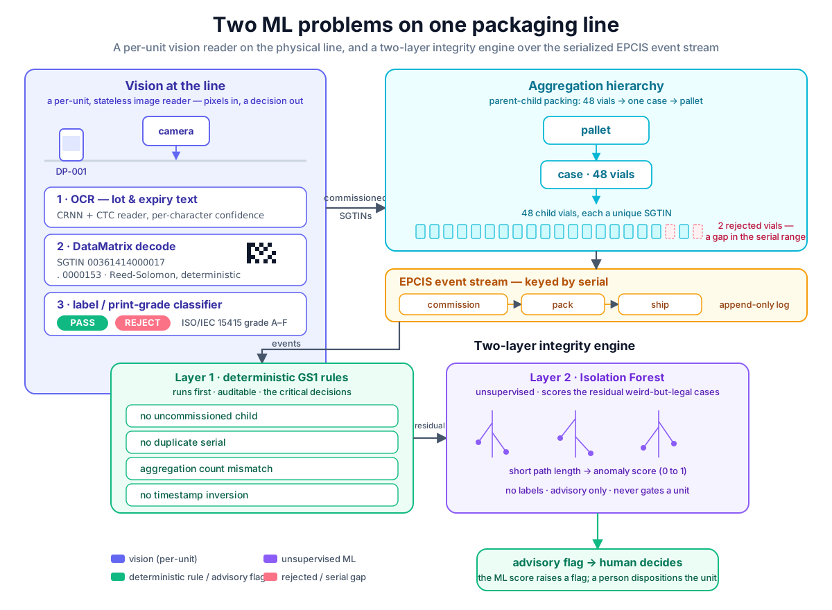The two ML problems of packaging side by side: a per-unit vision reader (OCR, DataMatrix decode, label grade) on the physical line, and a two-layer integrity engine over the serialized EPCIS event stream — deterministic GS1 rules first, an unsupervised Isolation Forest for the residual, with the ML score advisory and the human deciding. Original diagram by the authors, created with AI assistance.

A runnable model: serialization_anomaly.py

The example module examples/platform/ml/serialization_anomaly.py builds the whole integrity stack on the committed dataset examples/datasets/fill_events.csv. It commissions real SGTINs from the 480 filled vials of BATCH-2026-001 (keeping the leading zeros that pandas would otherwise destroy), excludes the two low_fill rejects so they are never commissioned, aggregates the survivors into cases of 48, runs the deterministic GS1 rule layer, and then scores the per-case feature table with an Isolation Forest. It runs standalone with no services.

# examples/platform/ml/serialization_anomaly.py (excerpt)
from pathlib import Path
import pandas as pd
from sklearn.ensemble import IsolationForest

DATA = Path(__file__).resolve().parents[3] / "examples" / "datasets"
VIALS_PER_CASE = 48          # vial -> case aggregation (illustrative hierarchy)


def commission_serials():
    """Each filled, NON-rejected vial is commissioned as an SGTIN at the fill line."""
    fe = pd.read_csv(DATA / "fill_events.csv", parse_dates=["ts"],
                     dtype={"vial_serial": str})        # keep GTIN/serial leading zeros
    fe["reject"] = fe["reject"].astype(str).str.strip().eq("True")
    fe[["gtin", "serial"]] = fe["vial_serial"].str.split(".", expand=True)
    commissioned = fe[~fe["reject"]].sort_values("ts").reset_index(drop=True)
    return fe, commissioned


def rule_checks(fe, cases):
    """Deterministic GS1/EPCIS invariants — NOT machine learning, and audited first."""
    findings = []
    if fe.loc[~fe.reject, "vial_serial"].duplicated().any():
        findings.append("duplicate_serial")
    phantom = set(fe.loc[fe.reject, "vial_serial"]) & set(fe.loc[~fe.reject, "vial_serial"])
    if phantom:
        findings.append(f"commissioned_rejected_unit x{len(phantom)}")
    short = cases[cases.n_vials != VIALS_PER_CASE]
    if len(short):
        findings.append(f"aggregation_count_mismatch x{len(short)} "
                        f"(e.g. {short.iloc[-1].case_id}={int(short.iloc[-1].n_vials)})")
    return findings or ["none"]


def score_anomalies(cases, contamination=0.08):
    """IsolationForest over per-case features -> advisory score for legal-but-strange cases."""
    feats = ["n_vials", "commission_span_s", "mean_fill_g", "fill_ratio", "serial_jump"]
    iso = IsolationForest(n_estimators=200, contamination=contamination, random_state=2026)
    X = cases[feats].to_numpy(float)
    iso.fit(X)
    cases = cases.copy()
    cases["anomaly_score"] = -iso.score_samples(X)   # higher = more anomalous
    cases["flag"] = iso.predict(X) == -1             # -1 = outlier
    return cases.sort_values("anomaly_score", ascending=False)

Running python platform/ml/serialization_anomaly.py prints the following block. Every number here is a verbatim run output over the real fill_events.csv — the GTIN, the 480/478 commissioned count, the two low_fill rejects, and the short final case — except the Isolation-Forest scores, which are deterministic given the seed but are an illustrative anomaly model over a clean campaign, not a learned fraud detector:

serialization / track-and-trace anomaly layer
  GTIN-14            : 00361414000017
  vials filled       : 480
  IPC rejects (not commissioned): 2 (['low_fill', 'low_fill'])
  serials commissioned: 478
  cases (48/case): 10 (last case is short: 46 vials)

-- rule layer (deterministic GS1/EPCIS invariants) --
  n_commissioned: 478
  n_rejected_not_commissioned: 2
  rule_findings: ['aggregation_count_mismatch x1 (e.g. CASE-009=46)']

-- ML layer (IsolationForest, advisory) — top scored cases --
 case_id  n_vials  fill_ratio  serial_jump  anomaly_score  flag
CASE-009       46       0.958            0          0.735  True
CASE-007       48       1.000            1          0.582 False
CASE-003       48       1.000            1          0.576 False
CASE-001       48       1.000            0          0.529 False
CASE-000       48       1.000            0          0.437 False

Read this output the way a serialization analyst would. The deterministic layer does the real work first: 478 of 480 vials are commissioned, the two low_fill rejects are correctly not commissioned (so they cannot become phantom units), and the one genuine structural defect — the final case CASE-009 holding 46 vials instead of 48 because the campaign does not divide evenly into cases — is caught by the exact, auditable aggregation_count_mismatch rule. Only then does the Isolation Forest run, and it independently surfaces the same CASE-009 as the top-scored, flagged outlier — agreeing with the rule but reaching it through statistics rather than logic. The two cases with serial_jump of 1 (CASE-007, CASE-003) score slightly higher than their peers because the rejected serials 0000152 and 0000342 left a one-unit gap that broke serial contiguity inside those cases — precisely the kind of weak structural signal the ML layer is there to notice. This is the whole design in miniature: rules catch the certain, ML scores the suspicious, and a human reads the flag.

Anatomy of one serialization event

A serialization event, like every artifact in this series, is not a bare serial number — it is a structured EPCIS record that ties the unit to what happened to it, where, when, and why, plus the model outputs and integrity verdicts that travel with it. Dissect one commissioning-then-packing event the way a track-and-trace reviewer would.

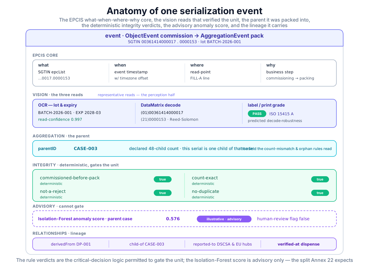One serialization event, fully unpacked: the EPCIS what-when-where-why core, the vision reads (OCR text with confidence, decoded DataMatrix, print grade) that physically verified the unit, the aggregation parent it belongs to, the deterministic integrity verdicts that are the critical-decision logic, the advisory Isolation-Forest anomaly score that is not, and the lineage tying the event to DP-001, its case, and the national hubs it is reported to. Original diagram by the authors, created with AI assistance.

Read the card top to bottom and the chapter is laid out as fields. The EPCIS core is the event proper — the what (the SGTIN epcList), when (the event timestamp), where (the read-point business location), and why (the business step: commissioning, then packing). The vision block carries what the camera physically verified: the OCR-read lot and expiry with a read-confidence (so a low-confidence read is flagged, not silently trusted), the decoded DataMatrix payload, and the label/print grade with its ISO/IEC 15415 letter grade. The aggregation block records the parent — CASE-003 and its 48-child count — making the parent-child relationship explicit and checkable. The integrity block holds the deterministic rule verdicts (commissioned-before-pack, not-a-reject, count-exact, no-duplicate), each marked deterministic because these are the critical-decision logic a regulator reads. The advisory block holds the Isolation-Forest anomaly score for the parent case, marked advisory and illustrative because under Annex 22 a probabilistic model cannot make the critical call. The violet relationships panel records lineage: this event derivedFrom DP-001, is child-of CASE-003, is reported-to the DSCSA and EU verification hubs, and is verified-at dispense — the last point in the running example's genealogy, where the SGTIN that began at fill is finally checked against the manufacturer's record before a patient receives the dose.

The unsolved part: rare, adversarial, and the saturation problem

Be honest about why serialization anomaly detection is harder than the clean demo suggests. The first difficulty is that the real anomalies are rare and adversarial. Unlike a drifting soft sensor, the most dangerous serialization anomalies — counterfactual cloning, diverted product re-introduced into the legitimate chain — are produced by an adversary who is actively trying to look normal. An Isolation Forest trained on legitimate traffic learns what normal looks like, but a sophisticated counterfeiter studies the same distribution and packs their fakes to sit comfortably inside it. Unsupervised anomaly detection raises the bar; it does not close the door, and treating its "no flag" as proof of authenticity is a category error.

The second difficulty is the alert-fatigue / saturation problem, the supply-chain cousin of AVI over-rejection. A track-and-trace system that flags too aggressively buries its real signals under a flood of benign oddities — a legitimately short final case, a re-work that updated parents correctly but unusually, a partner whose EPCIS clock is a few seconds off. Tune the Isolation Forest's contamination too high and human reviewers stop trusting the flags; tune it too low and the rare real fraud slips through. There is no clean operating point, and the only durable answer is the two-layer split this chapter insists on: keep the certain, auditable rules carrying the load, and use the ML score as a prioritizer for human attention, never as a gate.

The third difficulty is fragmentation. DSCSA and the EU FMD are different regimes with different event models, different hubs, and different verification flows, and a single global product crosses both. An anomaly model trained on one jurisdiction's event shapes does not transfer cleanly to the other, and the most interesting anomalies — a unit that appears in two countries' systems at once — are precisely the ones no single jurisdiction's data can see. Cross-jurisdiction anomaly detection requires data sharing that competitive and privacy pressures make genuinely hard, which is why most deployed anomaly work today lives inside one manufacturer's serialization repository, not across the chain.

What this chapter adds to the model suite

This chapter contributes examples/platform/ml/serialization_anomaly.py to the Book 5 example suite: a standalone module that commissions real SGTINs from fill_events.csv (correctly preserving the GTIN-14 and serial leading zeros), excludes the two low_fill IPC rejects from commissioning, aggregates the survivors into cases, runs a deterministic GS1/EPCIS rule layer (uncommissioned child, commissioned reject, aggregation-count mismatch, duplicate serial, timestamp inversion), and scores a per-case feature table with an unsupervised Isolation Forest. It coordinates with — and deliberately does not duplicate — the vision AVI sketch (vision_avi.py), which handles the perception half of packaging (the per-vial image classifier); this module handles the integrity-reasoning half (the serialized event stream). The commissioning counts, the GTIN, the two rejects, and the short final case are real committed-dataset facts; the Isolation-Forest scores are clearly labelled illustrative — they exercise a defensible anomaly model over a clean campaign rather than a learned fraud detector trained on confirmed fraud.

Why it matters

Packaging is the last place the digital thread touches the product, and it is where two regulatory regimes turn a manufacturing concern into a public-safety one. Get the vision right and the line auto-verifies print and codes at speed without burying operators in false rejects; get the integrity reasoning right and a counterfeit, a diversion, or a simple packing error is caught before it reaches a pharmacy shelf. The discipline this chapter insists on — deterministic rules carrying the critical decisions, ML scoring only the residual and only as advice — is not a limitation to apologize for. It is exactly the architecture the regulators are converging on, and it is what lets a manufacturer deploy machine learning here at all without putting a probabilistic model in the path of a unit's release. The SGTIN that began on a vial of BATCH-2026-001 at fill is the same identifier a pharmacist scans before a patient receives the dose; learning to keep that identifier honest is the quiet finale of the manufacturing half of the process.

In the real world

The vision half of packaging is genuinely production: deep-learning inspection of labels, print, and codes is sold and deployed by Stevanato, Syntegon, Brevetti CEA, Antares Vision, Cognex, and Körber, and it is the strongest production ML story in the whole fill-finish-and-packaging area — with the standing caveat that every headline accuracy and false-reject number is vendor / self-reported and the one fully validated public retrofit was a syringe line [3][4]. DataMatrix decoding and print grading against ISO/IEC 15415 are mature, standardized practice on every serialized line.

The track-and-trace anomaly half is more pilot than productized ML. DSCSA and EU FMD serialization themselves are fully production — every manufacturer commissions, aggregates, and reports EPCIS events today — but the deterministic rule layer does almost all the operational work, and learned anomaly detection over the event stream is an applied (pilot) idea that serialization-platform vendors are beginning to add rather than a settled, validated capability. The unsupervised-anomaly family this chapter uses (Isolation Forest, random forests) is the same one that appears in peer-reviewed biomanufacturing CPV work — CSL Behring and Aizon's "CPV of the Future" proof-of-concept — which grounds the method even though that work was on a microbial model system, not a serialization stream [6]. The broader frame is the one this whole book keeps returning to: the ISPE Pharma 4.0 reality is that production ML clusters in vision inspection and monitoring with a human in the loop, not in autonomous quality decisions, and a serialization anomaly score is squarely advisory under the FDA's 2023 Artificial Intelligence in Drug Manufacturing discussion paper and the draft Annex 22 [5][7]. And the cautionary tale sits one regime over: the April 2026 Purolea cGMP warning letter — the first to cite AI — flagged a firm using AI agents to generate specifications and master production records without quality-unit review, the exact opposite of the rules-first, ML-advisory discipline this chapter argues for [8].

Key terms

• Serialization — assigning a globally unique serial number to every saleable unit and tracking it through the supply chain, mandated by DSCSA (U.S.) and the FMD (EU).
• SGTIN (Serialized GTIN) — the unit identifier: a GTIN-14 (the product) plus a serial (the individual unit), e.g. 00361414000017.0000152; the join key for the whole track-and-trace record.
• DataMatrix — the 2D barcode symbology that carries the SGTIN, lot, and expiry on a vial; decoded deterministically with Reed-Solomon error correction.
• OCR (optical character recognition) — the learned vision task of reading the human-readable lot and expiry text, where flagging low-confidence reads matters more than reading clean text.
• Print-quality grading — scoring a printed code against ISO/IEC 15415 parameters (contrast, modulation, fixed-pattern damage) to predict whether it will still decode downstream.
• Commissioning — the act of declaring a serial to exist, attached to a real, accepted unit; a serial commissioned for a rejected unit is a phantom.
• Aggregation — recording the parent-child packing relationships (vial → bundle → case → pallet) so a pallet scan implies the serials beneath it.
• EPCIS — the GS1 standard for sharing supply-chain events; each event records what, when, where, why for a set of serials.
• DSCSA / FMD — the U.S. and EU track-and-trace regulations driving serialization and verification.
• Isolation Forest — an unsupervised, label-free anomaly detector that scores a point by how easily random splits isolate it; well suited to the rare, mostly-normal, weakly-labelled serialization regime.
• Two-layer integrity design — deterministic GS1/EPCIS rules for the auditable critical decisions, with an advisory ML anomaly score only for the residual of weird-but-legal cases.
• Alert saturation — the failure mode of an over-eager anomaly detector that buries real signals under benign flags, eroding reviewer trust.

Where this leads

The product is made, released, packed, and serialized; every vial of BATCH-2026-001 now carries an SGTIN that can be verified anywhere in the chain. What remains is getting it to the patient intact. The next chapter, Distribution: Cold-Chain Prediction and Demand Forecasting, leaves the factory entirely and learns the supply chain itself — predicting temperature excursions on a shipping lane before they happen, scoring route and partner risk, and forecasting demand so the right number of doses are made in the first place — closing the manufacturing spine where it finally meets the world.