Seed Train: Soft Sensing the Inoculum and Predicting Contamination Risk
📍 Where we are: Part III · Upstream, Learned — Chapter 10. The last chapter taught models to travel between scales; now those models meet their first real upstream job, the one the spine has always rushed past — the seed train that grows the inoculum and decides, on a clock nobody fully controls, whether the cells are ready to seed the big tank.
The seed train is the quiet stretch of the process. Between the thawed working cell bank and the production bioreactor sits a chain of ever-larger vessels — a shake flask, a wave bag, an N-2 then an N-1 seed reactor (the stages are numbered backward from the production tank, N) — each one growing the cells a little further until there are finally enough cells (the inoculum) to inoculate the production tank. It is also the most-skipped node of the series' shared process backbone — the spine this book and its four sisters all re-walk: every book in this series has glossed it, because nothing visibly happens there. No product is made; cells just divide. But that is exactly why it is a learning problem. The seed train is a race against two clocks — a growth clock you want to win and a contamination clock you want to avoid — and almost every decision in it is a prediction: how fast are the cells really growing, will they hit the target density in time, and is anything contaminating the culture before you commit it to a million-dollar batch.
This chapter treats the seed train as a first-class learned node. We build a growth-rate soft sensor for the small vessels where probes are scarce, a readiness-to-inoculate model that predicts when SEED-001 will be fit to seed the production reactor, and a contamination-risk classifier that watches for the metabolic and spectral fingerprints of bioburden long before a sterility test would catch it. And we are honest about the N-1 intensification decision — to run the last seed stage as a perfusion culture — which ML can inform but, under current regulation, cannot make alone.
Starting a sourdough culture, you do not bake the moment you mix flour and water. You wait, and you read cheap signals — how high it has risen, how it smells, how fast bubbles form — to judge whether the starter is active enough to bake with, and whether anything has gone off. The seed train is the same waiting game for cells. A growth-rate soft sensor reads cheap signals (how fast oxygen is consumed, how the medium turns) to estimate how fast the cells are dividing. A readiness model predicts whether the culture will be strong enough to use on schedule. And a contamination model sniffs for the off-smell — the metabolic wrongness that says something other than your cells is growing — before you commit the whole bake.
What this chapter covers
- The seed train as a distinct, learnable node, and why the spine keeps skipping it
- Growth-rate soft sensing in shake flasks and small seed bioreactors where instrumentation is thin
- Readiness-to-inoculate prediction — a classifier that flags a slow
SEED-001days before a fixed-calendar rule would - Contamination and bioburden risk prediction from metabolic and spectral signals, with honest evidence tiers
- N-1 perfusion intensification — what ML can inform about the decision and what it cannot decide
- The anatomy of one readiness prediction record, and the GMP (Good Manufacturing Practice) boundary it must respect
The seed train as a learning problem
A seed train is a sequence of expansion stages, conventionally numbered backward from the production bioreactor: the production stage is N, the last seed stage that inoculates it is N-1, the one before that N-2, and so on back to the thawed vial. Each stage has a job — multiply the cells by a target expansion factor (conventionally several-fold per passage at a fixed seeding density) while keeping them healthy — and a gate: whether the culture has reached a minimum viable cell density, at a viability floor, while still in exponential growth (the exponential phase is the stretch where the cells are dividing fastest, before nutrients run low and growth plateaus), so it can be split forward without carrying a plateauing, lactate-consuming culture into the next vessel — lactate consumption is the metabolic sign that the cells have left exponential growth, so such a culture would seed the next stage already past its prime. In our running example the gate is the inoculation of BATCH-2026-001 from SEED-001, the derivedFrom edge — the permanent "made-from" link that records a material's parentage — that Book 4 models as genealogy and Book 1 describes physically. The seed-train genealogy is real in the dataset: examples/datasets/lot_genealogy.csv records BATCH-2026-001 → SEED-001 → WCB-CHO-001, and each sibling batch carries its own seed (SEED-002 … SEED-006).
What makes this a learning problem rather than a logging problem is the clock. A seed stage that grows too slowly delays the whole campaign and can miss a scheduled production-suite slot; one that is pushed forward under-grown inoculates the production reactor at too low a density and skews the entire production run (14 days in our fed-batch simulator). So the operator wants to know, mid-stage, two things they cannot directly measure in real time: the current specific growth rate (μ, how fast the cells are actually dividing right now) and the readiness of the culture (whether it will cross its target density healthy and on time). Both are classic soft-sensing targets — soft sensing means estimating a quantity you cannot measure live from cheap signals you can — and both live in the worst possible data regime — small vessels with few probes, offline counts only once or twice a day, and a handful of historical seed trains to learn from. This is the cold-start, small-data reality the whole book keeps returning to, concentrated into the least-instrumented step in the plant.
The biology underneath is unforgiving in a useful way. A healthy CHO seed culture grows roughly exponentially during expansion, so as a first approximation viable cell density obeys X(t) = X0 · exp(μ · t) — where X is the cell density, X0 the starting density, t the elapsed time, and μ the specific growth rate that, in our simulator, tops out at MU_MAX = 0.58 per day (μ is a continuous rate, so a μ of 0.58/day means the population doubles roughly every 1.2 days — ln 2 / 0.58 — which works out to about a 79 percent net increase each day). μ is throttled by two Monod terms — the standard way to model how growth slows as a nutrient runs low, each term tied to a half-saturation constant, the concentration at which growth runs at half its maximum: glucose with K_GLC = 0.4 g/L and glutamine with K_GLN = 0.25 mM — plus a lactate-inhibition factor (model_fedbatch.py). That structure is what makes the seed stage predictable enough to learn: μ is not a free parameter, it is a function of the nutrient and by-product state, and the same online signals that move with the nutrient state therefore carry information about μ. The learning job is to invert that relationship from cheap measurements without ever seeing μ directly.
Where the training data lives, and why its meaning has to be modeled
A seed-train model is only as trustworthy as the dataset under it, and at seed scale that dataset is assembled from the least harmonized corner of the plant. The cheap signals the soft sensor leans on are born in three different systems that do not natively agree on what they are describing: the OUR and base-addition traces live in the process historian (the time-series store for in-process signals), the bench glucose/lactate/VCD counts live in the LIMS (Laboratory Information Management System), and the seeding density, vessel assignment, and shift events live in the MES (Manufacturing Execution System, the floor software that runs and records the run). Book 2's semantic-interoperability chapter shows the failure precisely: one physical temperature inside BR-101 is recorded by the historian, the MES, and the LIMS under three tag names, units, and timestamp formats, so a query for "all readings of this property for BATCH-2026-001" returns none of them automatically. A growth-rate feature table that silently joins temp_reactor to TIC101.PV on a guess is exactly how a seed model trains on a column that does not mean what its name says. The fix is the same one the data book prescribes — pin every signal to a controlled vocabulary so the join is on meaning, not on a string — and it is what lets a feature be pulled by its semantic identity rather than a fragile column header.
That harmonization has a standard shape. ISA-95 (the model that names equipment, materials, and the batch hierarchy) and B2MML (its XML serialization) give the seed vessels, the inoculation event, and the lot a shared vocabulary across the historian/MES/LIMS seam, and OPC UA (the modern industrial-data protocol whose information model carries that structure on the wire) is how the historian receives the N-1 reactor's tags already typed rather than as bare numbers. A seed-train feature pipeline built on that grounding is reproducible because the join is specified, not guessed.
The deeper grounding is ontological, and it is the seed train's own genealogy that supplies it. The derivedFrom edge introduced above is not decoration — it is the grouping key the model's cross-validation must respect. Each seed train and the batch it inoculates form one lineage (BATCH-2026-001 → SEED-001 → SEEDFLASK-001 → WCB-CHO-001, the chain Book 4 makes transitive), and readings from the same lineage are correlated — same WCB vial, same medium lot, same operators — so a random train/test split that scatters one seed's timepoints across both halves leaks information and inflates the score. Grouping the cross-validation by the derivedFrom lineage — a leave-one-seed-train-out split — is what makes the AUROC an honest estimate of performance on the next seed rather than on a memorized one. The lineage edge that exists for recall traceability turns out to be the correct partition for learning.
And one BFO (Basic Formal Ontology) distinction the upper model draws keeps the feature table itself coherent. Book 4 types the seed culture run as an occurrent (a happening that unfolds over the stage and is gone) and the bench count of viable cell density as a continuant quality measured at an instant — different aisles, joined by an edge, never one node wearing both types. That cut is why a soft-sensor feature can be unambiguously stamped: this μ-anchor is a quality measured at time t on the culture, not a property of the run as a whole. Confuse the two and the anchoring breaks — you cannot say which instant a count pins the trace to. The semantic backbone is not overhead on the model; it is what makes the model's inputs mean one thing.
Growth-rate soft sensing in the small vessels
In the production bioreactor, a Raman probe and a battery of online sensors make titer and metabolite soft sensing routine. The seed train is harsher. Early stages are shake flasks and rocking bags with almost no in-line instrumentation; even the N-1 seed reactor carries fewer probes than the production tank. The signals you reliably do have are the cheap ones — dissolved oxygen and its controller's response, the oxygen uptake rate (OUR) inferred from gas balancing, base addition to hold pH, agitation power, and the offline glucose/lactate/VCD bench samples that arrive twice a day. The soft sensor's job is to turn those into a live growth-rate estimate.
The physics gives the soft sensor its backbone, which is why this is naturally a hybrid model rather than a pure black box. In an exponential-growth seed culture, viable cell density follows X(t) = X0 · exp(μ · t), so the specific growth rate over an interval is just the slope of log-density against time:
μ ≈ [ ln X(t2) − ln X(t1) ] / (t2 − t1)
That equation is exact but useless minute-to-minute, because X only arrives twice a day from the bench. The soft sensor's trick is to interpolate μ between bench counts using the continuous signals that co-vary with it. The chain of proxies is mechanistic, not hand-waved. Oxygen uptake rate scales with viable biomass, so OUR is a near-real-time proxy for X. The rate of base addition tracks lactate production, which in the growth phase tracks glucose consumption — in the simulator lactate is produced at a yield Y_LAC_GLC = 0.35 of glucose uptake while μ is high (mu > 0.15) and is consumed once growth slows, so the sign of the lactate slope itself is a growth-phase indicator. That base-addition-tracks-lactate proxy holds only in the growth phase; once the culture shifts to lactate consumption the pH rises (possibly calling for acid, not base), so the proxy weakens or inverts exactly as the lactate slope changes sign. And the in-line glucose probe falls at a rate Q_GLC per unit biomass, so the glucose-consumption slope is a direct readout of how much living biomass is drawing down the medium.
A model that maps (OUR, base rate, glucose-consumption slope, agitation power) onto μ — anchored at each bench count so it cannot drift far from ground truth — gives a continuous growth-rate trace from sparse measurements. The right way to state the estimation objective is a regularized least-squares fit on the residual μ that the mechanistic backbone does not already explain: minimize Σ (μ̂(features) − μ_anchor)² at the bench-count timepoints, plus a smoothness penalty between them, so the trace is forced through the few real counts and interpolated, not invented, in the gaps. In our simulator the metabolic coupling is explicit — glucose uptake and lactate yield both scale with viable biomass — so the in-line glucose probe and the online tags carry a genuine, learnable signal about how fast the cells are growing rather than a coincidence the model has overfit.
This is the growth-rate version of the titer soft sensor from Book 2's machine-learning chapter and Book 3's analytics chapter, and the same honesty applies: the estimate is only as good as its anchor, and between bench counts the soft sensor is extrapolating a slope, so its confidence interval — the band of plausible values around the estimate — must widen the further it sits from the last real count. A growth-rate reading without an uncertainty band is a number you should not trust to schedule a batch. The feature engineering that makes the difference is the same discipline as everywhere upstream — rate features (slopes, not levels) over short rolling windows, every feature anchored to the last validated bench measurement, and a hard rule that the model output never overrides the count it was trained to track.
Readiness-to-inoculate: predicting the gate
Growth rate is the instantaneous question; readiness is the forecast. The operator does not only want "how fast are the cells dividing now," they want "will this culture be fit to seed the production reactor on the day we planned, so we can book the media prep and the production-suite crew." That is a classification problem at heart: given the culture's early trajectory, will it clear the inoculation gate — a minimum viable cell density at a viability floor, while still in exponential growth, on schedule — or will it fall short? Framing readiness as a binary outcome (ready / not ready) rather than a bare hour is what lets a scheduler flag a slow seed days earlier than a fixed-calendar rule, with a calibrated probability instead of a guess — it is the sourdough question made precise: is the starter active enough to bake with on the day you planned to bake, not merely active.
The features that drive readiness are the ones a process scientist would name without a model: the early specific growth rate μ (a fast culture clears the gate), the lag phase (a long post-thaw lag pushes everything later), the viability (an unhealthy culture is unfit regardless of count), and the day-3 lactate (over-production of lactate flags a stressed, inefficiently metabolizing culture that will plateau early). The honest model is a small, interpretable one — a logistic regression, which squashes a weighted sum of the features through the sigmoid (an S-shaped curve that maps any number to a probability between 0 and 1) to predict a yes/no outcome — on standardized features, because at seed scale there are only a handful of historical trains, the relationships are close to monotone (each feature pushes readiness consistently one way — always up or always down), and such an interpretable model is far easier to defend to the quality unit (the QA department that signs off on every release) than a tree ensemble (a model that averages many decision trees) that found a spurious split — a rule that fits noise in the small training set rather than real biology. The readiness probability is P(ready) = σ(w·z + b), where σ is that sigmoid, z the standardized features, w the learned per-feature weights, and b an offset — and the learned weights are the explanation: a positive weight on μ and viability, a negative weight on lag and lactate, each in units the reviewer can sanity-check against process knowledge.
There are richer framings for plants with more history. Regression on remaining time maps the current state directly onto "hours until target VCD," answering "when" with a point estimate and an interval. Mechanistic extrapolation with a learned correction projects the logistic/exponential growth curve forward from the current state, then applies a small learned residual that captures the systematic ways this cell line, in these vessels, deviates from the textbook curve (a longer lag after thaw, an earlier plateau at high density). This is the hybrid pattern again, and it extrapolates far more safely than a pure regressor when only a few seed trains exist. But all three framings share the same boundary, and it is the one that matters most.
The value is operational, not regulatory — readiness prediction schedules the inoculation; it does not authorize it. The authorization still rests on the actual at-line VCD and viability measured at the gate, reviewed by a human. The model buys foresight (book the suite a day early, or flag a slow culture in time to intervene), not the decision itself. That boundary is the recurring theme of upstream ML: models advise the schedule; the release of cells forward is human-in-the-loop.
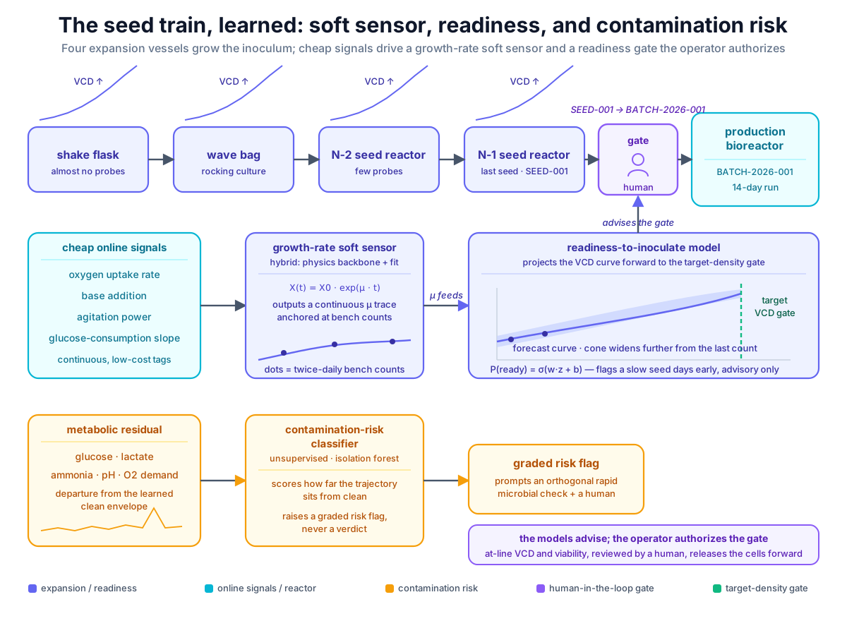 The seed train, learned: cheap online signals feed a growth-rate soft sensor anchored at sparse bench counts; a readiness model projects the density curve forward to the inoculation gate with widening uncertainty; a contamination-risk classifier watches the metabolic residual in parallel; and the SEED-001 → BATCH-2026-001 inoculation stays a human-authorized gate that the models only inform.
Original diagram by the authors, created with AI assistance.
The seed train, learned: cheap online signals feed a growth-rate soft sensor anchored at sparse bench counts; a readiness model projects the density curve forward to the inoculation gate with widening uncertainty; a contamination-risk classifier watches the metabolic residual in parallel; and the SEED-001 → BATCH-2026-001 inoculation stays a human-authorized gate that the models only inform.
Original diagram by the authors, created with AI assistance.
A readiness and growth-rate model in code
The chapter's runnable artifact is examples/platform/ml/seed_ready.py. It builds the readiness-to-inoculate classifier on a synthetic cohort of 300 seed cultures — synthetic, and tagged as such, because real seed-train labels are precisely the thing a plant has only a few of. Each simulated seed carries the four features a process scientist would read at day 3: the early specific growth rate μ, the lag phase in hours, the viability, and the day-3 lactate. The label is whether the seed is ready — fast growth, short lag, healthy, and not over-producing lactate — and the readiness outcome is generated from a logistic relationship over those features so the experiment has a known signal to recover. We use scikit-learn, the canonical open-source Python machine-learning library for this scale of problem [1], and a logistic regression because the cohort is small, the relationships are close to monotone, and the learned coefficients are the explanation a reviewer needs:
# examples/platform/ml/seed_ready.py — inoculation-readiness classifier (synthetic cohort)
import numpy as np
from sklearn.linear_model import LogisticRegression
from sklearn.metrics import roc_auc_score
from sklearn.model_selection import train_test_split
from sklearn.preprocessing import StandardScaler

N = 300

def make_seeds(seed=2026):
    rng = np.random.default_rng(seed)
    mu = rng.normal(0.55, 0.10, N)                 # early specific growth rate (1/day)
    lag_h = rng.normal(18, 6, N).clip(2, 40)       # lag phase (h)
    viab = rng.normal(95, 3, N).clip(80, 99.5)     # viability %
    lactate = rng.normal(1.2, 0.5, N).clip(0.1, 3) # day-3 lactate g/L
    X = np.column_stack([mu, lag_h, viab, lactate])
    # ready = fast growth, short lag, healthy, not over-producing lactate
    logit = 6 * (mu - 0.5) - 0.08 * (lag_h - 18) + 0.15 * (viab - 92) - 1.2 * (lactate - 1.2)
    ready = (rng.random(N) < 1 / (1 + np.exp(-logit))).astype(int)
    return X, ready

def main() -> dict:
    X, ready = make_seeds()
    Xtr, Xte, ytr, yte = train_test_split(X, ready, test_size=0.35, random_state=0, stratify=ready)
    sc = StandardScaler().fit(Xtr)
    clf = LogisticRegression(max_iter=1000).fit(sc.transform(Xtr), ytr)
    auroc = roc_auc_score(yte, clf.predict_proba(sc.transform(Xte))[:, 1])
    print("Seed-train inoculation-readiness model (synthetic 300-seed cohort)")
    print(f"  readiness classifier AUROC = {auroc:.3f}")
    print(f"  ready fraction in cohort = {ready.mean():.2f}")
    assert auroc > 0.70, "readiness model should clear AUROC 0.70"
    return {"auroc": float(auroc)}
A few details earn their place. The features are standardized before fitting — each feature recentred to mean 0 and unit spread — so the coefficients are directly comparable and the regularization treats them on the same scale; a seed-scale model with four differently-scaled inputs (independent here by construction, though potentially correlated in real data) is exactly where an unscaled fit misleads. The split is stratified on the readiness label — a train/test split (here holding out 35 percent of the cohort to score on) that keeps the same ready/not-ready ratio in both halves — because the cohort is imbalanced (more ready than not) and an unstratified split can hand the test set too few of the positives (the ready cultures) to score honestly. And the metric is AUROC (area under the receiver-operating-characteristic curve), not accuracy: a readiness flag is a ranking decision (which seeds are most at risk of missing the gate), and AUROC measures exactly that ranking quality independent of where you set the threshold. The threshold itself is a downstream, operational choice — set it conservatively and you investigate more cultures than strictly necessary; set it loosely and you miss slow seeds — and it should be tuned on the cost of a missed slow seed (a delayed or under-grown batch) against the cost of a needless investigation.
One discipline the code does not show but a governed deployment needs is a completeness gate on the inputs, and it is the same mechanism Book 4 uses for lot release. A readiness prediction made from an incomplete or out-of-range feature row is worse than no prediction — a missing day-3 lactate or a viability of 120 percent silently corrupts the score. Book 4 models the release decision as a SHACL shape (the Shapes Constraint Language, which validates that graph data has the required structure) precisely because a missing required result is a failure, now — not an open question. The same shape, pointed at the model's input rather than the release panel, is the right pre-flight check: every one of the four features present (sh:minCount 1), singular (sh:maxCount 1), the right datatype, and inside its plausible range (sh:minInclusive / sh:maxInclusive), with the anchoring bench count present and recent. SHACL guards the seam between the historian, the MES, and the LIMS — exactly where a dropped row or a duplicated count slips in — so the model never scores a row the data systems left half-built. The release gate's completeness guarantee is the training-and-inference data-quality guarantee, reused.
Run it and it prints the real output from RUN_OUTPUTS.txt:
### seed_ready.py ###
Seed-train inoculation-readiness model (synthetic 300-seed cohort)
  readiness classifier AUROC = 0.750
  ready fraction in cohort = 0.65
Read like a process engineer: on a 300-seed synthetic cohort the readiness classifier ranks seeds by their chance of clearing the gate at AUROC 0.750 — on a scale where 0.5 is a coin flip and 1.0 is a perfect ranking — comfortably above the 0.70 floor the assertion guards, with 65 percent of the cohort actually ready. That is deliberately not a heroic number. AUROC 0.75 is "useful triage, not an oracle" — it will reliably surface the slowest, least-healthy cultures days earlier than a fixed-calendar rule, which is the entire operational point, but it is nowhere near tight enough to authorize an inoculation. The honest reading is that early features carry real but partial information about a gate that depends on the full trajectory, and a model trained on a few hundred synthetic seeds should not pretend otherwise. The assertion assert auroc > 0.70 exists so the claim cannot silently rot — if a future change broke the seed signal, CI would fail loudly, exactly as the Book 3 soft-sensor script guards its own R².
Contamination and bioburden risk prediction
The second clock is the dangerous one. A seed train that grows perfectly but is contaminated — a stray bacterium, a fungus, a mycoplasma (a tiny wall-less bacterium notorious for contaminating cell cultures undetected) — can ruin not just the seed but the production batch it inoculates, and the standard sterility and bioburden tests are slow: a compendial sterility test (one run by the official pharmacopoeia method, USP / Ph. Eur.) famously takes up to 14 days, far longer than a seed stage lasts. So by the time a culture-based test confirms contamination, the contaminated inoculum may already be in the production tank. The learning question is whether cheaper, faster signals carry an early fingerprint of contamination, so a risk can be flagged in time to hold the gate.
There are two families of approach, and the evidence behind them sits at different maturity tiers — this book uses two conventions on every claim: a maturity tag ((research) / (pilot) / (production)) saying how far a technique has travelled toward routine plant use, and an evidence rung (press-release-only → vendor-self-reported → peer-reviewed-self-authored → peer-reviewed-independent) saying how trustworthy the number behind it is:
- Metabolic-signature anomaly detection. A contaminating organism metabolizes differently from CHO cells — it can spike glucose consumption, shift the lactate or ammonia trajectory, or change pH and oxygen demand in ways that diverge from the learned "clean" envelope. The right tool is unsupervised: train on clean seed trains only and flag any culture whose metabolic trajectory leaves the normal cloud. An isolation forest does this by randomly partitioning the feature space and scoring how few splits it takes to isolate a point, averaged over an ensemble of random trees — anomalies isolate in fewer splits, giving an anomaly score (a mean path length, not a single split count) with no need for contaminated examples. A one-class SVM (support vector machine) instead learns a boundary that encloses the clean data and scores distance outside it. This is the multivariate-monitoring idea pointed at sterility instead of quality, and the same machinery (isolation forest for batch-phase anomalies, random forest for control actions) is what Aizon, with the Universitat Autonoma de Barcelona, demonstrated for continued process verification — though that proof-of-concept ran on a Pichia pastoris (a yeast) model system, not a mammalian CHO seed train, so it is (research), peer-reviewed-self-authored, and should not be over-read as a deployed contamination detector [2].
- Spectroscopic identification. Raman (an optical probe that reads a sample's chemical fingerprint from scattered laser light) and UV-absorbance spectra carry organism-specific fingerprints, and supervised classifiers have been shown to identify microbial contamination from spectra in research settings. A Raman-based convolutional neural network classified twelve common pharmaceutical contaminant organisms — including mixtures with CHO cells — at 95–100 percent accuracy [3], and a machine-learning-aided UV-absorbance one-class SVM trained on sterile MSC supernatant detected contamination at roughly 10 CFU/mL (colony-forming units per millilitre — a low, sensitive detection limit) across seven strains in cell-therapy products [4]. Both are (research) demonstrations — peer-reviewed-independent — and neither is a GMP-deployed rapid sterility method; the regulatory bar for replacing a compendial sterility test is very high.
One caveat sharpens the honesty: mycoplasma is the case the metabolic anomaly detector is least likely to catch. Unlike a fast-growing bacterium or fungus, mycoplasma often grows slowly, leaves little overt metabolic signature, and may not turbid the culture at all — which is exactly why an organism-specific orthogonal test (rapid PCR / nucleic-acid amplification) remains mandatory and why the anomaly score can only ever be a prompt, never a clearance.
The honest framing is risk, not verdict. A contamination-risk model produces a graded anomaly score — "this culture's metabolic trajectory is anomalous, investigate" — that prompts an orthogonal (independent, different-principle) rapid microbiological method (a validated RMM under the compendial standards USP <1223> / Ph. Eur. 5.1.6 — ATP-bioluminescence, a growth-based rapid sterility method, or a targeted PCR), a flow-cytometry viability check, and a human decision. It does not, and under current regulation cannot, replace the sterility test or autonomously fail a lot. And the base rate is brutal: real contamination events are rare, so a supervised "detect contamination" classifier has almost no positive examples to learn from — which is exactly why the unsupervised "departure from clean" framing is the more honest one, and why the score is a prompt for an orthogonal test, never a standalone verdict. Its value is the same as the readiness model's: foresight bought cheaply, in time to hold the gate before the contaminated inoculum moves forward.
Anatomy of one readiness prediction
A readiness prediction is not a bare probability. Like every artifact in this series, its value is in what travels with the number — the inputs that produced it, the model and data version behind it, the uncertainty around it, and the gate measurement that will eventually grade it. The record seed_ready.py would persist for SEED-001, dissected field by field, is the seed-train analogue of the soft-sensor prediction record and the same governed object the MLOps chapter will track for drift.
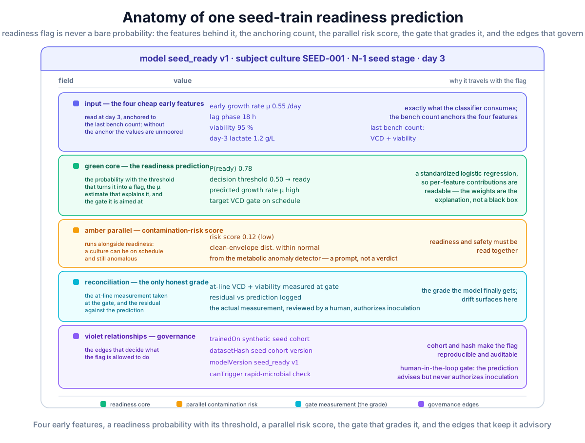 One readiness prediction is a whole record: the early features and their anchoring bench count, the readiness probability with its threshold and the growth-rate estimate, the parallel contamination-risk score, the gate measurement that will grade it, and the relationships that make it governable — including the human-in-the-loop gate the prediction advises but never authorizes.
Original diagram by the authors, created with AI assistance.
One readiness prediction is a whole record: the early features and their anchoring bench count, the readiness probability with its threshold and the growth-rate estimate, the parallel contamination-risk score, the gate measurement that will grade it, and the relationships that make it governable — including the human-in-the-loop gate the prediction advises but never authorizes.
Original diagram by the authors, created with AI assistance.
Read the card top to bottom and the chapter's argument is laid out as fields. The input rows are the four cheap, early features the classifier actually consumes — μ, lag, viability, day-3 lactate — plus the last bench count of VCD and viability that anchors them; without that anchor the feature values are unmoored. The green core is the prediction proper: the readiness probability paired with the operating threshold that turns it into a flag (so a reader can see how close to the line this culture sits), the growth-rate estimate that explains why the probability landed where it did, and the target VCD gate the forecast is aimed at. Because the model is a standardized logistic regression, the card can carry the per-feature contribution — the signed weight times the standardized value — so the reviewer sees that, say, a long lag drove the "not ready" flag rather than a black-box pronouncement.
The amber parallel block is the contamination-risk score running alongside, because readiness and safety must be read together — a culture can be perfectly on schedule and still anomalous. The reconciliation rows hold the gate measurement (the at-line VCD and viability the operator actually measures at inoculation) and the residual against the prediction, the only honest grade the model ever gets. And the violet relationships panel records governance: the seed cohort it trained on, the dataset hash, the model version, the rapid-microbial check the risk score can trigger, and — the field that matters most — the human-in-the-loop inoculation gate the prediction advises but does not authorize.
The N-1 perfusion intensification decision
The most consequential seed-train decision of the last decade is N-1 perfusion intensification: running the final seed stage not as a batch but as a perfusion culture — continuously flowing fresh medium in and spent medium out (rather than filling the vessel once and harvesting at the end) while bleeding cells (drawing off a fraction to keep the density from running away) — to reach a very high density, so the production reactor can be inoculated at five to ten times the conventional cell density. A high-density inoculum shortens the production growth phase and can materially lift volumetric productivity (product made per litre of reactor per day) — it is one of the real workhorses of process intensification. The fed-batch core (model_fedbatch.py, with DAYS = 14) is the simulated data we actually have; the intensified perfusion path is described qualitatively here rather than backed by a perfusion module in the suite.
The decision is genuinely multi-dimensional, which is what makes it a modeling target rather than a rule of thumb. The lever is the cell-specific perfusion rate (CSPR) — fresh medium delivered per cell per day — together with the bleed rate that holds the high-density steady state. The two levers divide the labor: the bleed rate sets the steady-state density — growth balanced against the dilution of bleed plus perfusion — while the CSPR sets how much fresh medium each cell sees per day, and so governs both nutrient sufficiency and the dominant cost of the stage. Too low a CSPR starves the dense culture and crashes viability; too high a CSPR burns medium (the dominant cost of a perfusion stage) for no benefit. The objective is to reach the target high-density inoculum, on schedule, at the lowest medium cost and without driving up the metabolic by-products that propagate into the production run. That is a constrained optimization over an operation that runs for weeks, with a slow and expensive feedback loop — exactly the shape that invites ML, and exactly the shape where ML's role must be stated carefully.
Where does ML fit? It informs the decision and the operation, but it does not make it:
- Informing the decision. Whether and how to intensify is a process-development question — and that is the home of Bayesian optimization and the hybrid digital twins that predict how a high-density inoculum will propagate into the production run. A perfusion-process hybrid model — a mechanistic core predicting viable cell density and other states feeding a shallow neural network that predicts mAb-specific productivity — can predict the cell-density trajectory and the downstream effect on titer under a candidate CSPR/feed policy, shrinking the experiments needed to qualify the intensified seed [5].
- Running the stage. A perfusion seed reactor runs for weeks at near-steady state, which turns the per-batch readiness question into a continuous one — the CSPR and the bleed must be held in band, and a soft sensor that tracks density and a drift monitor that watches the steady state become daily operational tools rather than per-batch ones. The most advanced demonstration here comes from DataHow, with Sartorius and Merck: an autonomous perfusion cultivation on a 24-parallel ambr250 mini-bioreactor platform, driven by Bayesian optimal experimental design and a cognitive digital twin of step-wise Gaussian-process models. It shows what is possible at PD scale — a 27-day proof of concept with roughly 20 days run by the autonomous agent — though the authors themselves stress the gap between robotic capability and device autonomy: it is (research), peer-reviewed, a development-scale proof of concept, explicitly not GMP [6]. Note that DataHow is an independent company in this collaboration, not a Sartorius subsidiary.
And a correction the field gets wrong often enough to name: National Resilience's widely cited "+50 percent titer" perfusion story is a PAT-plus-manual-feed-optimization result — PAT (process analytical technology) being in-line measurement, here used to guide manual feeding, not ML — reported in a vendor press release — Resilience used the 908 Devices REBEL at-line media analyzer to add back only depleted nutrients — not an ML deployment, and it should never be presented as evidence of machine learning lifting titer [7]. The intensification gains are real; attributing them to ML is not.
The unsolved part: anchoring a soft sensor when the anchor barely exists
Every soft sensor in this book leans on a slow reference to keep it honest. The seed train pushes that dependence to its breaking point. In the production bioreactor the offline reference arrives once or twice a day; in a shake-flask seed stage it may arrive once a day at best, and the early N-2 stages may have only a single count before they pass forward. A growth-rate soft sensor anchored on one or two points is extrapolating almost the entire time, and a readiness model built on a few historical seed trains — even our 300-seed cohort is synthetic precisely because a real plant has nothing like 300 labeled trains — is the deepest reach into the cold-start regime the upstream ever asks for.
This makes two failures genuinely hard. The first is silent growth-rate drift: between the rare counts, a soft sensor that has begun to over-read μ (because of a probe shift, a new medium lot, a longer-than-usual lag after thaw) looks identical to one that is right, and the readiness forecast it feeds is confidently wrong. There is no second reference in the gap to catch it, and the cheap online signals it relies on can drift with the error — a fouled DO probe biases both the OUR proxy and the μ estimate in the same direction, so the soft sensor's own inputs conspire to hide the drift. Because that bias is common-mode, the drift monitor cannot read the same channel it is meant to police: it has to be built on a proxy orthogonal to the suspected fault — cross-checking the OUR-derived μ against the base-addition and glucose-slope estimates, or a model innovation test — since a monitor reading the same fouled input is blind to the drift it shares. The second is the contamination base-rate problem, which we met earlier and which the seed train makes structural rather than incidental: because real contamination is rare, no amount of additional seed-train history will hand a supervised classifier the positive examples it lacks — the unsupervised "departure from clean" framing is not a temporary workaround for thin data, it is the permanent shape of the problem, and even its flag stays a prompt for an orthogonal test.
The transfer-learning and Bayesian-prior approaches that the rest of the book leans on are the most promising path — hybrid Gaussian-process models with learned entity-embedding vectors can borrow the growth and metabolic priors learned from related cell lines and prior campaigns to compensate for this line's thin history [8] — but none of them substitutes for the reference data the seed train structurally cannot provide. A prior sharpens a thin posterior; it does not manufacture the one or two counts the stage will never run. The honest seed-train soft sensor is one that knows how little it knows: wide intervals, anchored hard to whatever counts exist, a drift monitor on its own inputs, and deferring every consequential decision to the human at the gate.
What this chapter adds to the model suite
This chapter contributes examples/platform/ml/seed_ready.py to the Book 5 example suite: the inoculation-readiness classifier, built with scikit-learn over a synthetic 300-seed cohort, with a CI assertion that the readiness signal stays predictive (AUROC above 0.70). It is the upstream counterpart of Book 3's soft_sensor.py — same discipline (a tagged-synthetic dataset, a stratified held-out split, a guarded metric), aimed at readiness instead of titer. The growth-rate soft sensor and the contamination-risk classifier sketched here share machinery the rest of the suite builds out in full — the hybrid backbone from the hybrid-models chapter and the anomaly-detection used in the QC and release chapter — so this chapter contributes the seed-stage framing and features rather than a second, duplicated detector. Together they make the seed train a node the model suite can actually run on, not a gap between cell-line development and the bioreactor.
Why it matters
The seed train is the cheapest place to prevent the most expensive failure. A growth-rate soft sensor and a readiness flag turn the seed stage from a fixed wait into a managed schedule — booking the production suite a day early when the culture is racing, or catching a slow culture in time to intervene rather than inoculating under-grown. A contamination-risk flag two days ahead of the sterility result is the difference between scrapping a seed flask and scrapping BATCH-2026-001. And modeling the N-1 intensification decision with a hybrid twin is how a plant qualifies a high-density inoculum on a handful of runs instead of a campaign of them. Get the seed train right and the production bioreactor inherits a healthy, on-schedule, sterility-confidenced inoculum; skip it — as the spine usually does — and the most data-rich step downstream is built on the least-watched step upstream.
In the real world
Seed-train ML is real but early, and it clusters where the rest of upstream ML clusters: monitoring and soft sensing, not autonomous control. Growth-rate and metabolite soft sensing in seed and production vessels is (production) practice via the same Raman-plus-PLS and multivariate platforms (Sartorius SIMCA / SIMCA-online, BioPAT) — where PLS (partial least squares) is the regression that turns a Raman spectrum into a concentration reading that monitor the production tank. N-1 perfusion intensification is a (production) process technology across the industry, but the ML around it — hybrid twins to design it, soft sensors to run it — is (pilot) to (research): the DataHow/Sartorius/Merck autonomous-perfusion work is a development-scale proof of concept, peer-reviewed but explicitly not GMP [6]. Contamination prediction is the least mature: Raman and UV deep-learning contamination identification are (research) demonstrations [3][4], and metabolic anomaly detection for process monitoring is a (production) technique (isolation forest, random forest) but has not been qualified as a rapid sterility method. The throughline is the one FDA's 2023 discussion paper and the ISPE Pharma 4.0 survey keep finding: AI/ML in this part of the plant has the most pilots and the fewest scaled deployments, concentrated in human-in-the-loop monitoring rather than autonomous decisions about a critical quality attribute (CQA) — a property like purity or potency that must stay in range to keep the product safe and effective [9]. The seed train, learned, is a place where models earn trust by advising the gate — not by holding it.
Key terms
- Seed train — the chain of expansion stages (vial → flask → N-2 → N-1) that grows cells from the working cell bank to the density needed to inoculate the production bioreactor.
- N-1 / N stage — the numbering convention counting backward from the production stage (N); N-1 is the last seed stage that inoculates it.
- Specific growth rate (μ) — the instantaneous rate of cell division; the slope of log viable-cell-density against time, throttled by nutrient (Monod) and by-product-inhibition terms.
- Soft sensor — a model that estimates a quantity you cannot measure live (here μ or readiness) from cheap signals you can, validated against a slow offline reference.
- Growth-rate soft sensor — a soft sensor that estimates μ continuously from cheap online signals (OUR, base addition, agitation power), anchored at sparse offline counts.
- Readiness-to-inoculate — a classifier that flags whether a seed culture will clear its target-density gate on schedule, used to schedule the inoculation; it advises but does not authorize the gate.
- AUROC — area under the receiver-operating-characteristic curve; measures how well a model ranks positives above negatives independent of the decision threshold.
- N-1 perfusion intensification — running the last seed stage as a perfusion culture to reach high density, so the production reactor is inoculated at much higher cell density.
- CSPR (cell-specific perfusion rate) — the fresh-medium perfusion rate per cell, the key control variable of a perfusion seed stage.
- Contamination / bioburden risk prediction — flagging the metabolic or spectral fingerprint of contamination earlier than a slow sterility test, as a graded risk that prompts an orthogonal check.
- Metabolic-signature anomaly detection — unsupervised flagging of a culture whose metabolite trajectory departs from the learned clean envelope (isolation forest, one-class SVM).
- Human-in-the-loop gate — the principle that the model advises the inoculation decision while a human, using the actual at-line measurement, authorizes it.
- CQA (critical quality attribute) — a product property (such as purity or potency) that must stay in range to keep the drug safe and effective; the regulatory bar an autonomous model would have to clear, and does not yet.
derivedFromlineage — the transitive "made-from" edge (BATCH-2026-001 → SEED-001 → … → WCB-CHO-001) that roots every lot in its cell bank; here it doubles as the grouping key for a leave-one-seed-train-out cross-validation so the AUROC is not inflated by leakage.- Semantic interoperability — the work of making the historian's, MES's, and LIMS's differently-named records of one physical signal mean the same thing, so a seed-train feature is joined on meaning (via ISA-95 / a controlled vocabulary), not a fragile column name.
- SHACL input gate — the same closed-world completeness shape that gates lot release, pointed at the model's input row to reject a feature that is missing, duplicated, or out of range before it can corrupt a prediction.
- Continuant / occurrent (BFO) — the upper-ontology cut that types the seed run as a happening and a bench count as a quality measured at an instant, keeping a measurement distinct from the run it was taken during.
Where this leads
The seed train hands a healthy, on-schedule, sterility-confidenced inoculum forward across the SEED-001 → BATCH-2026-001 gate. The next chapter, The Production Bioreactor: Soft Sensors, Closed-Loop Control, and the Digital Twin, is where the soft-sensing we sketched at seed scale becomes the most mature ML in upstream — Raman-plus-PLS titer and metabolite prediction, closed-loop glucose control, and the hybrid digital twin of the 14-day run that the whole upstream has been building toward.