UF/DF and Drug Substance: Soft-Sensing Concentration and Excipients

📍 Where we are: Part IV · Downstream, Learned — Chapter 16. Polishing chromatography handed downstream a pure pool of antibody, monomeric and charge-correct, but dilute and sitting in the wrong buffer. This chapter learns the final transformation: squeezing that pool to its drug-substance concentration and exchanging its buffer — and producing DS-001, the lot where every release critical quality attribute (CQA) — the measured properties a regulator ties to a drug's safety and efficacy — is at last measured.

The molecule is now pure. What it is not yet is finished. After polishing, the antibody is a clean but dilute stream — a few grams per litre, dissolved in the elution buffer of the last column, which is nothing like the buffer a patient's dose needs. The job of the last downstream unit operation, ultrafiltration/diafiltration (UF/DF), is two things at once: push water through a membrane to concentrate the protein up to its drug-substance target (often tens of grams per litre for a modern high-concentration mAb), and wash out the old process buffer, replacing it with the formulation buffer the molecule will live in (diafiltration). When the membrane finally stops, what comes off it is the drug substance — the bulk material the rest of the supply chain treats as the product — and in our running example that is the lot DS-001 (a lot is one discrete, traceable batch of material), deriving from PApool-001 (the Protein A capture pool earlier in the purification train) and the whole genealogy behind it.

UF/DF is where the learning lens meets a deceptively simple-looking step, and it is also where the release CQAs we have been chasing since the bioreactor finally get measured. Two numbers govern the operation — how concentrated the protein is, and how much old buffer is left — and neither of them has a fast, cheap, GMP-grade (Good Manufacturing Practice — the binding quality-system rules drug makers must follow) inline assay (a laboratory measurement of a quality attribute) that is easy to trust. So the chapter is, once more, a soft-sensing chapter — inferring a quantity that is slow or expensive to measure directly from cheap signals that are always available: predict the concentration and the excipient state from the cheap signals the skid already carries, predict when diafiltration is done, and flag the excursions that ruin an otherwise-finished batch.

The simple version

Think of reducing a sauce and then changing its seasoning. You boil off water until it is thick enough (that is concentration), then you keep adding fresh stock and boiling it down again, over and over, until the old salty broth is almost entirely replaced by the new one (that is diafiltration). The hard part is knowing two things without stopping to taste: how thick the sauce is right now, and how much of the old broth is still in there. A UF/DF soft sensor is the cook who can read both off the look and feel of the pot — the colour, the way it coats a spoon — so they know exactly when it is done and when something has gone wrong, without ladling out a sample and waiting. And there is a way to ruin it: reduce too hard and too fast, and a skin forms and scorches against the bottom of the pot — it will not redissolve, and it taints the batch. A good cook reads that the sauce is fighting back and eases off before it burns. A UF/DF excursion monitor watches for exactly that skin forming against the membrane.

What this chapter covers

• Framing UF/DF as two coupled soft-sensing problems — concentration (a moving target as water leaves) and excipient/buffer state (a moving target as buffer is exchanged), and why the offline assays for both are too slow to control on.
• Inline concentration soft sensing — variable-pathlength UV280, refractive index, and Raman fused into one g/L number, and why a linear model is the right tool here, not a deep net.
• The diafiltration endpoint — a learned endpoint predictor in log-residual space that stops at the right diavolume instead of a fixed number, called a fraction of a diavolume early.
• Excursion detection — gel-layer/concentration-polarization faults, the stagnant-film flux model they violate, and how a one-sided residual against that physics flags a UF/DF run going wrong.
• The DS-001 node — where the release CQAs (monomer, host-cell protein (HCP) — a process impurity carried over from the production cells — the rest of the panel) are finally measured, how the soft sensors connect to them, and the contrasting fate of a sibling lot, BATCH-2026-004, that fails the same panel on HCP.
• A runnable module, examples/platform/ml/ufdf_endpoint.py, its verbatim output, and the anatomy of one UF/DF endpoint record field by field.
• The honest open problem: high concentration breaks the linear assumptions, and the reference is the slowest of all.

UF/DF is two soft-sensing problems wearing one skid

It helps to be precise about the physics before the learning. A tangential-flow filtration (TFF) skid — a self-contained, plumbed assembly of pump, membrane, and probes on a frame — pumps the protein pool across a membrane whose pores pass water and small solutes (buffer salts, sugars) but retain the large antibody. The fluid that passes through the membrane is the permeate; what is held back is the retentate. In the ultrafiltration phase you simply remove permeate, so the retained volume shrinks and the protein concentration climbs in proportion to the volume-reduction factor (VRF). The mass balance is exact when the membrane fully retains the protein (the sieving coefficient S is the fraction of a solute that passes into the permeate — S ≈ 0 means the membrane holds it all back, S ≈ 1 means it passes freely; here S ≈ 0 for the retained antibody): the protein mass behind the membrane is conserved, so

c(t) · V(t) = c0 · V0        ⇒        c(t) = c0 · V0 / V(t) = c0 · VRF

Concentrate from 8 L to 1.6 L and you have multiplied concentration five-fold. In the diafiltration phase you hold volume constant — adding fresh formulation buffer at exactly the rate permeate leaves — so concentration stays put while the old buffer ions are progressively flushed out and replaced. For a freely-permeating small solute (sieving coefficient S ≈ 1) in an ideal, well-mixed retentate, the solute mass balance over a differential volume of permeate dVp is V · dc = −S · c · dVp; integrating at constant V and substituting the diavolume DV = Vp / V (the number of retentate-volumes of fresh buffer exchanged) gives the textbook exponential wash-out:

C_residual / C_initial  =  exp(−S · DV)   →   exp(−DV)   for S = 1

so roughly three diavolumes clears about 95% of the old buffer, five clears about 99%, and seven about 99.9% (these follow directly from the exponential: exp(−3) ≈ 0.05 residual = 95% cleared, exp(−5) ≈ 0.01 = 99%, exp(−7) ≈ 0.001 = 99.9%). That clean exponential is the backbone every UF/DF model leans on — and it is exactly the kind of trustworthy physics that, in the small-data regime of bioprocess, you should never throw away in favour of a black box. (The same algebra exposes the two ways the ideal breaks: incomplete mixing makes S look effectively below 1 and slows the wash-out, while protein-bound or charge-partitioned counter-ions make the apparent decay non-single-exponential — both of which the learned version below absorbs as a fitted rate constant rather than the textbook's S = 1.)

A real high-concentration mAb drug-substance recipe is usually three phases, not two: UF1 pre-concentrates the dilute pool, DF exchanges buffer at a manageable intermediate working concentration, and UF2 over-concentrates to the final DS target — typically followed by a buffer flush and recovery rinse to sweep protein out of the system hold-up (the volume of product left stranded in the tubing and dead spaces of the skid). The soft sensors therefore operate at different points on the trajectory (diafiltration runs below the final concentration the UV will eventually read), and final-concentration accuracy depends on system hold-up and flush recovery, not on the UV read alone. Even so, the two governing quantities move on different schedules. Protein concentration rises during UF and is then held during DF; the excipient state is unchanged during UF and decays during DF. Both matter for release: the drug substance has a target concentration with a tolerance, and a buffer/excipient specification (residual old buffer washed out, formulation excipients dialled in). And both are awkward to measure live. Concentration is classically measured by pulling a sample and running an offline A280 (absorbance at 280 nm, the protein concentration readout detailed in the next section) or a slow protein assay; the excipient/buffer state is measured by osmolality, ion chromatography, or pH/conductivity benchtop checks. Each takes long enough that, by the time the lab reports, the membrane has moved on. That gap — a value that matters now against a confirmation that arrives later — is the same measurement gap that created the titer soft sensor upstream, transplanted to the very last downstream step.

Inline concentration: variable-pathlength UV, refractive index, and why linear wins

The single most important inline measurement in UF/DF is protein concentration, and the production-grade way to get it is variable-pathlength ultraviolet (VPE/VPX) spectroscopy. The chemistry is Beer-Lambert: absorbance at 280 nm is proportional to protein concentration times the optical pathlength, A = ε · c · ℓ, where ε (the mass extinction coefficient) is a fixed per-protein constant that says how strongly that protein absorbs — for a typical mAb ε ≈ 1.42 L·g⁻¹·cm⁻¹ (the value the companion module uses), so once ε is known a single absorbance reading pins the concentration. At a few grams per litre a normal 1 cm cuvette works fine, but a high-concentration drug substance at tens of g/L would drive A well past 2–3 AU (absorbance units), into the detector's non-linear tail dominated by stray light — light reaching the detector by paths other than through the sample — where so little light gets through the sample that this leakage dominates and the relation stops being a line. The variable-pathlength trick is to shorten the optical path — Repligen's variable-pathlength technology sweeps ℓ continuously down to roughly 5 µm — and pick the pathlength that keeps A inside the calibrated linear window (conventionally A under 1.5 AU — the conservative calibrated ceiling, with visible non-linearity setting in by 2–3 AU). The instrument then back-computes c = A / (ε · ℓ), so a single cell reads concentration from about 0.1 mg/mL to past 250 mg/mL without ever diluting the retentate. Repligen's FlowVPX/FlowVPE is the commercial embodiment of this, integrated inline with the KrosFlo KR2i automated TFF system to monitor and control UF/DF by concentration rather than by retentate weight, with the analytics line having come to Repligen via its March 2025 acquisition of 908 Devices' bioprocessing analytics portfolio [1] (production, vendor-self-reported — every claim in this book carries such a tag for how mature the deployment is and how independent the evidence is; see the maturity and evidence-tier conventions).

Two more cheap inline signals carry the same information from a different angle. Refractive index rises almost linearly with dissolved protein — the Lorentz-Lorenz relation linearizes to a near-constant specific refractive-index increment dn/dc ≈ 0.185 mL/g for protein, so n ≈ n_buffer + (dn/dc) · c — making RI a robust, drift-resistant secondary that, crucially, does not saturate the way an optical absorbance does. Raman spectroscopy carries protein concentration and excipient identity in one spectrum — the excipients are the inactive formulation ingredients (buffer salts, sugars, surfactants) that surround the antibody (the amide-I and amide-III bands, two spectral features produced by the protein backbone, track protein; distinct buffer-species peaks track the excipients), which is why it has become the research workhorse for UF/DF monitoring of multiple attributes at once. The learning task is to fuse these into a single calibrated concentration. Concretely, that fusion is a tiny supervised regression: stack the inline channels into a feature row x = [A280, n, …], collect a handful of grounding samples whose true c came from an offline A280, and fit the weights w that minimize Σ (cᵢ − wᵀxᵢ)² — ordinary least squares when the channels carry independent information, partial least squares (PLS) when they are collinear — when the channels move together and so duplicate each other's information (UV and RI are, since both track the same c), which makes the plain least-squares weights unstable and is what PLS is built to handle. With only two channels and hundreds of grounding points the collinearity is harmless — OLS simply distributes the weight between UV and RI — so the companion module uses ordinary least squares; PLS earns its keep when you add Raman's hundreds of collinear wavenumbers, where a latent-variable projection (a handful of components chosen by cross-validation) is what keeps the calibration stable. Two grounding points already pin the slope and intercept; a dozen pin them with margin.

And here is the crucial methodological point this chapter wants to make loudly: for concentration, the right model is a small linear one, not a deep network. Beer-Lambert is genuinely linear in c; the Lorentz-Lorenz RI relation is genuinely linear in c; the physics already tells you the functional form. A PLS or ordinary-least-squares calibration on a handful of grounding samples will match or beat a neural network here, will extrapolate far more safely (a fitted line behaves predictably one step past its last training point; a deep net can do anything off-distribution), and — decisively for GMP — is trivially explainable to a reviewer: two coefficients with physical units they can sanity-check against the literature ε and dn/dc. Reaching for a deep net on a problem the physics has already linearized is the cardinal small-data sin this whole book warns against. (Deep learning earns its place where the relationship is genuinely nonlinear and the data is rich — high-concentration viscosity, charge-variant pooling — not on a Beer-Lambert line.)

The excipient/buffer state is the harder of the two, because conductivity and refractive index respond to all the ions, not just the old buffer you are trying to remove. During diafiltration the bulk conductivity moves monotonically from the old-buffer endpoint toward the new-buffer endpoint, but a single mid-exchange reading is ambiguous about the residual old-buffer fraction unless the calibration knows both endpoints — which is exactly what Raman's species specificity resolves. A diafiltration soft sensor for the residual old-buffer fraction is therefore a model that disentangles the formulation buffer being added from the process buffer being removed: in the linear case it subtracts the known new-buffer conductivity baseline and rescales the remainder against the pure-old-buffer reading. This is exactly where Raman's chemical specificity (it can tell two buffer species apart by their distinct spectral fingerprints, not just their lumped ionic strength) beats a bulk property like conductivity, and where a multivariate model earns its keep.

One subtlety the wash-out math hides: at the high protein concentration of a modern drug substance, the equilibrated excipient and pH state inside the retentate is not simply the diafiltration buffer's composition. Charged excipients and buffer species partition unequally across the membrane by the Donnan effect (the charged protein, held back by the membrane, electrostatically tilts the equilibrium distribution of small ions across it), and the protein itself excludes volume (its molecules physically occupy space the small solutes cannot, so the same amount of excipient sits in less free water), so the final formulated levels are offset from the DF-buffer levels. That is why formulators deliberately diafilter into an offset buffer and why the excipient soft sensor — and the offline osmolality and pH reference behind it — must be grounded against the equilibrated retentate, not the buffer it was fed.

The diafiltration endpoint: stop at the right diavolume, not a fixed number

A naive UF/DF recipe diafilters a fixed number of diavolumes — "always run 7 DV" — chosen with a generous safety margin so the wash-out is guaranteed even on a bad day. That works, but it is wasteful: every extra diavolume is fresh buffer, processing time, and another window for the membrane to foul or the protein to aggregate at the gel layer. A learning plant instead predicts the endpoint: it watches the residual old-buffer signal decay and stops as soon as the model says the residual is reliably under spec, with a confidence margin.

The endpoint problem is a soft sensor plus a threshold crossing, and the trick that makes it work early is to do it in log-residual space. The features are the inline conductivity and Raman trajectory over diavolumes; the modelled quantity is the residual old-buffer fraction f(DV); the endpoint is the first diavolume at which the predicted residual — not a single noisy probe reading — falls under the wash-out specification f_spec. Because the underlying decay is exponential, f(DV) ≈ exp(−k·DV), taking the log makes it a straight line: ln f = ln(exp(−k·DV)) = −k·DV — the logarithm is the exact inverse of the exponential, so the curve flattens into a line whose slope is −k, and a line is trivial to fit and extrapolate. Fit k by least squares to the early part of the curve (the first one or two diavolumes, where the signal-to-noise is best because plenty of old buffer is still present), then solve the line for the crossing:

DV_endpoint  =  −ln(f_spec) / k

So a model fit to the first diavolume can call the stop a fraction of a diavolume in advance, with a prediction interval that comes straight from the regression's standard error on k. Because the line is fit, not just read off, the regression also hands you an honest error bar on k, and therefore on the predicted stopping point: that error bar is exactly the safety margin a reviewer wants you to build in before trusting an early call. The pay-off is concrete: stopping at a model-predicted 3.0 diavolumes instead of a recipe-mandated 7 is more than a factor-of-two reduction in diafiltration buffer (and a comparable saving in time, insofar as permeate flux holds steady — DF time tracks diavolumes only while flux does not decline as fouling builds), with the residual still demonstrably under spec.

This is also where UF/DF connects to the AI-enhanced continued-process-verification (CPV) work the field is publishing: treating each UF/DF run's trajectory (flux, transmembrane pressure, concentration, conductivity) as a multivariate object and monitoring it batch-to-batch with the same multivariate-SPC tooling the open-source analytics chapter defines in full — building a principal-component model of past good ("golden") batches and charting two summary alarms (Hotelling's T² and the squared-prediction-error Q, the in-model and off-model distance from that envelope) against control limits — so a run that is drifting away from the envelope is flagged early, aligned to FDA and EU GMP Annex 15 lifecycle process-control expectations [2] (pilot, peer-reviewed-independent). The endpoint model and the CPV monitor are two faces of the same trajectory model: one calls the stop, the other says whether the trajectory getting there looked normal.

Excursion detection: when the membrane fights back

UF/DF looks gentle but has a signature failure mode the soft sensors must guard against: concentration polarization and the gel layer. As water is pulled through the membrane, protein piles up against its surface faster than it can diffuse back into the bulk, forming a concentrated, viscous boundary layer. The stagnant-film model captures the normal regime: flux J (the volume of liquid passing through a unit of membrane area per unit time) is J = k_m · ln(c_wall / c_bulk), where c_wall is the protein concentration right at the membrane surface and c_bulk the concentration out in the well-mixed pool, and k_m is the back-diffusion mass-transfer coefficient (how fast protein piled at the wall can diffuse back into the bulk) set by crossflow — the tangential sweep of feed across the membrane face that scours the wall layer (written k_m to keep it distinct from the diafiltration decay-rate constant k of the previous section). Past a critical flux the wall concentration c_wall saturates at a gel concentration c_gel and the membrane chokes — flux collapses, transmembrane pressure (TMP) climbs without a flux gain (the pressure-independent plateau), and in the worst case protein at the wall denatures or aggregates, quietly seeding the high-molecular-weight species that the SEC release assay will later catch. The excursion is invisible to a single concentration reading; it shows up as a relationship going wrong — flux falling faster than the concentration ramp says it should, or TMP rising without a corresponding gain in concentration.

That makes excursion detection a natural fit for the same residual-against-physics idea used elsewhere in this book. You have a mechanistic expectation — the flux-versus-TMP line, the J = k_m · ln(c_wall/c_bulk) polarization curve, concentration versus VRF — and you watch the residual r = J_observed − J_expected(TMP, c) between what the physics predicts and what the skid is actually doing. Because gel-layer fouling only ever suppresses flux, the right detector is one-sided: alarm when the standardized residual r / σ_r drops past a negative control limit (below −3, say), not on two-sided deviation, since a positive residual is just favourable mass transfer. Read r / σ_r in words: it is the residual measured in units of its own normal scatter σ_r, so a value past −3 means the flux has fallen more than three times further below the physics line than a healthy run ever wanders — the same three-sigma trip the control charts elsewhere in this book use. The same one-sided residual also covers progressive membrane fouling over a run (rising TMP at constant flux, falling normalized permeability), the most common real UF/DF excursion of all; operationally an operator charts it with a pre/post-run Normalized Water Permeability (NWP) measurement plus TMP excursion limits during the run — the standard membrane fouling/integrity guardrail a reviewer actually looks for.

And because gel-layer fouling builds rather than spikes, the robust trigger is not a single point past −3 but a one-sided CUSUM (or EWMA) on the standardized residual crossing its decision interval — a run-length rule that ignores single noisy dips and fires only on a sustained drift. A persistent negative residual is the fault signature: gel-layer formation, a fouling membrane, a failing pump, or a temperature excursion changing viscosity. This is structurally identical to the chromatography trajectory monitoring of the previous chapter — a multivariate trajectory, a learned or physics-based normal envelope, and an alarm on departure — applied to a TFF skid instead of a column. It is also squarely in the human-in-the-loop, advisory category the regulators endorse: the model flags the excursion and a human decides whether to intervene, hold, or investigate.

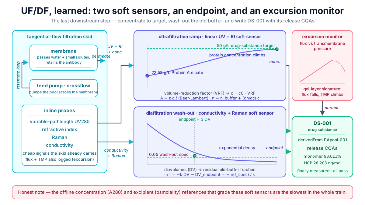The last downstream step, learned: a linear concentration soft sensor reads the ultrafiltration ramp, an excipient soft sensor reads the diafiltration wash-out and predicts the endpoint, and an excursion monitor watches the flux-pressure relationship for the gel layer — together they produce DS-001, the drug-substance lot that finally carries the release CQAs of the running example. Original diagram by the authors, created with AI assistance.

A runnable model: ufdf_endpoint.py

The example module examples/platform/ml/ufdf_endpoint.py builds both soft sensors and the endpoint predictor, grounded in the running example's real numbers. It starts the concentration ramp from the actual Protein A eluate titer of BATCH-2026-001 — 22.58 g/L, read straight from protein_a_summary.csv (eluate_titer_g_L), and ends at the released drug-substance CQAs read from hplc_results.csv (monomer 98.611%, HCP 28.203 ng/mg). The UF/DF step itself is not in the simulator, so the concentration ramp and the diafiltration wash-out curve are surrogate physics — Beer-Lambert UV, a membrane mass balance, and the textbook exponential decay — clearly labeled illustrative. The soft-sensor method is real; only the trajectory it is fit on is synthetic.

The structure mirrors the chapter's argument exactly. simulate_ufdf lays down the two-phase ground truth — a UF ramp c = c0 · VRF and a DF wash-out excipient_frac = exp(−DV) — then observes it through three noisy inline channels that encode the real physics constants: a variable-pathlength UV proxy at ε = 1.42 L·g⁻¹·cm⁻¹, a refractive index at n = 1.3330 + 1.8e-4 · c, and a conductivity at 2.5 + 13.0 · excipient_frac mS/cm. fit_concentration_softsensor then fits the two-term linear fusion (uv280 + refractive_index → g/L) the section above derived and scores it on a held-out split, and predict_df_endpoint implements exactly the endpoint method this chapter describes: it fits the excipient soft sensor on a held-out split, takes the log of the predicted residual fraction, fits the decay rate k by least squares on the first one-to-two diavolumes, solves the line for the crossing, and reports a 95% confidence interval from the standard error — with a deterministic full-curve first-crossing kept alongside as a cross-check. ds_release_summary reads the real release panel back from hplc_results.csv.

# examples/platform/ml/ufdf_endpoint.py  (faithful excerpt)
DS_TARGET_G_L = 50.0          # high-concentration mAb DS target (illustrative)
EXCIPIENT_SPEC = 0.05         # residual old-buffer fraction to clear by diafiltration


def simulate_ufdf(c0: float, n: int = 400) -> pd.DataFrame:
    """Surrogate UF concentration ramp + DF wash-out (illustrative physics)."""
    # concentration (UF) phase: c = c0 * VRF as volume is reduced
    vrf = np.linspace(1.0, DS_TARGET_G_L / c0, n // 2)
    conc = c0 * vrf
    # diafiltration (DF) phase: residual old buffer decays as exp(-DV)
    dv = np.linspace(0.0, 8.0, n - n // 2)
    excip_df = np.exp(-dv)                                    # ideal wash-out decay
    df = pd.DataFrame({...})                                  # phase, diavolume, protein_g_L, excipient_frac
    eps = 1.42                                                # mAb A280 extinction (L/g/cm)
    df["uv280_AU_per_cm"]    = eps * df.protein_g_L + noise   # variable-pathlength UV
    df["refractive_index"]   = 1.3330 + 1.8e-4 * df.protein_g_L + noise
    df["conductivity_mS_cm"] = 2.5 + 13.0 * df.excipient_frac + noise
    return df


def fit_concentration_softsensor(df):
    """Linear is right here: Beer-Lambert UV + refractive index -> g/L."""
    X = df[["uv280_AU_per_cm", "refractive_index"]].to_numpy()
    # scored on a HELD-OUT split, not in-sample: the number a reviewer sees
    Xtr, Xte, ytr, yte = train_test_split(X, df["protein_g_L"].to_numpy(), test_size=0.3)
    reg = LinearRegression().fit(Xtr, ytr)
    ...


def predict_df_endpoint(df, spec=EXCIPIENT_SPEC, early_dv=2.0):
    """Endpoint by EARLY-WINDOW log-residual extrapolation, with a CI."""
    dfp = df[df.phase == "DF"]
    # excipient soft sensor (held-out): inline conductivity -> residual fraction
    reg = LinearRegression().fit(dfp[["conductivity_mS_cm"]], dfp["excipient_frac"])
    f_pred = reg.predict(...).clip(1e-4, None)
    # fit ln f = b0 + b1*DV on the FIRST one-to-two DV only, then solve the line:
    early = dfp[dfp.diavolume <= early_dv]
    b0, b1 = np.linalg.lstsq(...)          # least squares in log-residual space
    dv_end = (np.log(spec) - b0) / b1      # extrapolated crossing, before reaching it
    se_end = ...                           # 95% CI from the standard error on (b0, b1)
    return dv_end, se_end                  # plus a deterministic first-crossing cross-check

Running python platform/ml/ufdf_endpoint.py prints the block below verbatim. The starting eluate (22.58 g/L) and the DS-001 release CQAs are real committed dataset values; the soft-sensor R² (scored on a held-out split) and the endpoint diavolume are computed on the illustrative surrogate trajectory:

UF/DF starts from the real Protein A eluate: 22.58 g/L -> DS target 50.0 g/L (illustrative)
concentration soft sensor (UV280 + RI -> g/L): R2=0.9997 RMSE=0.1452 g/L, final 49.89 g/L   # illustrative
diafiltration endpoint (early-window log-residual extrapolation): excipient<= 0.05 reached at 3.0 diavolumes [95% CI 2.99-3.01], decay k=0.998/DV   # illustrative
  cross-check: deterministic first crossing at 3.02 DV; excipient soft sensor R2=0.9997 (held-out)
DS-001 release CQAs (real): monomer 98.611%  HCP 28.203 ng/mg  all_pass=True
ASSERT ok: inline UV+RI recover protein concentration and the wash-out endpoint is extrapolated with a confidence interval (illustrative).

Read the output as the chapter's argument made executable. The concentration soft sensor recovers the protein concentration almost perfectly (R² 0.9997, RMSE 0.1452 g/L) — R² is the fraction of the concentration variation the model explains, where 1.0 is perfect and 0 is no better than always guessing the average, and RMSE (root-mean-square error) is the typical miss in real units, here about 0.15 g/L. Crucially that R² is scored on a held-out split, not in-sample — that is, graded only on data points the model never saw while it was being fit, the one honest test of whether it generalises rather than memorises — so it is the number a reviewer would see on rows the fit never touched. A near-perfect held-out R² is exactly what you expect when the model matches the physics, and the RMSE of about a seventh of a gram per litre is just the injected sensor noise, not model bias; a held-out split lands in the same place precisely because a Beer-Lambert line has nothing to overfit. (That is itself a small lesson: a deep net on this problem could memorise the noise and post a deceptively lower training error, then fail off-distribution.) The diafiltration endpoint lands at 3.0 diavolumes with a tight 95% interval of 2.99–3.01 — far short of a recipe-mandated 7 — extrapolated from the early-window log-residual fit (decay rate k = 0.998/DV); a deterministic full-curve first-crossing at 3.02 DV is reported alongside as a cross-check, and the two agreeing to a hundredth of a diavolume is the evidence the early call is trustworthy. The early endpoint saves more than half the buffer (and a comparable slice of time) the conservative recipe would have spent, with the residual still demonstrably under the 5% wash-out spec. And the DS-001 line closes the genealogy: the drug substance carries the real release CQAs, monomer 98.611% and HCP 28.203 ng/mg, all of which pass. (The module's assert conc["r2"] > 0.95 and assert lo <= endpoint <= hi are the executable claims — if a future refactor breaks the linear fusion or pushes the endpoint outside its own interval, the run fails loudly rather than shipping a silently wrong soft sensor.)

Anatomy of one UF/DF endpoint record

A UF/DF batch does not end with a bare "stopped at 3 DV." Like every artifact in this series, the endpoint is a structured record that ties the stop decision to the trajectory that justified it, the soft-sensor predictions that called it, the specifications it was checked against, and the drug-substance lot it produces. Dissect it the way a manufacturing-science reviewer would before disposition.

One UF/DF endpoint, fully unpacked: the inline trajectory that fed it, the concentration and excipient soft-sensor predictions that called the stop, the specifications and excursion check it satisfied, the real release CQAs the resulting DS-001 lot carries, and the lineage tying it to PApool-001 and forward to fill-finish — with the honest note that the references that grade it are the slowest in the whole train. Original diagram by the authors, created with AI assistance.

Read top to bottom and the chapter is laid out as fields. The header names the producing model and version — ufdf_endpoint v1, the locked artifact a change-control plan would version — and the lot it produces, DS-001, derivedFrom PApool-001.

The input block is the inline trajectory, and every field in it is an inline signal, which is the whole reason a soft sensor is possible here:

• variable-pathlength UV280 — the primary concentration channel, A = ε·c·ℓ with ℓ swept to keep A in the linear window; feeds the concentration soft sensor.
• refractive index — the saturation-proof secondary concentration channel, n ≈ n_buffer + (dn/dc)·c; fused with UV280.
• Raman — the multi-attribute channel that carries both protein and excipient identity; the chemical-specificity input the excipient soft sensor leans on.
• conductivity — the bulk excipient/buffer-state channel that drives the diafiltration wash-out fit.
• flux and transmembrane pressure — the pair the excursion monitor differences against the polarization physics; they do not feed the concentration or endpoint models, only the gel-layer detector.

The green core is the decision the record exists to justify:

• final concentration 49.89 g/L against the 50 g/L target — the soft-sensor read at the end of the UF ramp (illustrative).
• endpoint 3.02 diavolumes — the deterministic first DV where the predicted residual crossed spec, the cross-check on the early-window log-residual call of 3.0 DV (illustrative).
• residual excipient fraction under the 0.05 wash-out spec — the quantity the endpoint was called on.

The constraints row writes down what the endpoint must satisfy — the concentration tolerance around the 50 g/L target and the under-0.05 wash-out specification — so a reviewer can see why the model stopped where it did, not just that it stopped. The excursion row carries the flux-TMP residual flag, the one-sided gel-layer early warning, recorded as normal on this run. The CQA-handoff row is what makes this the release-defining node: the real monomer 98.611% and HCP 28.203 ng/mg results that DS-001 carries forward, both inside spec (monomer spec 95–100%, HCP under 100 ng/mg) and both PASS. The violet relationships panel records lineage: this record derivedFrom PApool-001, produces DS-001, feeds formulation and fill-finish, reconciledWith the offline A280 and osmolality references, and retrains_when the residual against those references drifts past its control limit. This record is the ML-side view of the same drug-substance lot that Book 4's ontology models as its DS-001 node — Book 5 reads the CQAs in this book's ng/mg convention and tracks the soft-sensor predictions and the endpoint that called the stop, while Book 4 validates the lot's release panel as formal SHACL shapes; the two are the same lot seen through each book's lens, not byte-identical copies of every attribute.

The contrast that makes the CQA-handoff row matter is a sibling lot. Where DS-001 (BATCH-2026-001) clears the panel at HCP 28.203 ng/mg, BATCH-2026-004 carries a near-identical monomer (98.687%) but an HCP — host-cell protein, the residual cell-derived impurity the panel caps — of 128 ng/mg against the same 100 ng/mg ceiling, an out-of-specification (OOS) result. A UF/DF soft sensor cannot save that lot: HCP is a carry-through impurity decided upstream at capture and polishing, and UF/DF only concentrates whatever entered it. But the record format is exactly what an OOS investigation reads — same fields, same references — to confirm the UF/DF step itself ran normally (no excursion flag, endpoint on schedule) and therefore exonerate it, pointing the investigation upstream. That is the quiet value of writing the endpoint down as a structured record rather than a number: it is evidence in both directions.

Why the ontology is what makes this soft sensor trustworthy

It is worth being precise about why those derivedFrom/produces/reconciledWith edges are not decoration. They are the semantic layer that lets the soft sensor be FAIR — Findable, Accessible, Interoperable, Reusable — and, more pointedly, trustworthy. Four of the panel's release attributes — monomer, HCP, the endpoint, the concentration — are only meaningful if every consumer of this record agrees on what each one is, and that agreement is what an ontology supplies. Book 4 gives every quantity a stable IRI (Internationalized Resource Identifier — a globally unique web name for a concept, the ontology counterpart of a fragile spreadsheet column header), so the model's input is bp:proteinConcMgPerMl carrying its qudt:unit, not a column called conc that one historian export spells conc_g_L and another protein_concentration. A feature pulled by its IRI cannot be silently swapped for the wrong column or the wrong unit — the most common cause of a soft sensor that validates in the lab and drifts in the plant.

The same release-gate SHACL shape that Book 4 uses to decide whether DS-001 may claim release also earns a second life as the training-data gate. bp:ReleaseShape says the monomer result must be present, singular, xsd:float, and at or above 95.0; the HCP result present and at or below its limit; the concentration inside its 45–55 mg/mL window. Run that same shape over a candidate training row and you have a closed-world guarantee that the model's inputs are complete and in range — a missing or duplicated CQA is caught as a validation failure now, exactly as a missing sterility test fails a lot, rather than slipping into the fit as a silent gap an open-world query would have shrugged at. The asymmetry the ML book keeps returning to — a reasoned graph constraining a guessing model — is concrete here: the shape that gates the lot also gates the data the lot's predictor learns from.

Two further edges do load-bearing work the column-name view cannot. First, the continuant/occurrent cut Book 4 draws under BFO keeps the measurement (the 49.89 g/L final concentration, a quality that inheres in the material) distinct from the run (the UF/DF process that produced it, an occurrent that happened once and is gone). Fusing them — the careless mistake of one fuzzy "UF/DF" node — would make it impossible to say the same skid ran a different batch last week, or to attach the endpoint to the run while attaching the concentration to the lot; the soft sensor's prediction and the process that justified it stay two linked things, not one. Second, the bp:derivedFrom lineage spine — declared transitive, walked by the GraphRAG (bp:derivedFrom)+ traversal Book 4 builds — is the grouping key for leave-one-batch-out cross-validation: honest scoring requires holding whole physical batches out, and that grouping is only possible because bp:BATCH-2026-001 is one global, stable identity across the historian, the LIMS, and this release record. A graph that named one batch four ways, or fused two with an over-eager owl:sameAs, would break the group boundary and leak the held-out set into training — which is why the held-out R² of 0.9997 is only as honest as the identity discipline behind the split. Identity, FAIR features, and the SHACL gate are not Book 4's concern bolted onto Book 5; they are the conditions under which this chapter's R² means anything at all. The same verified graph is then what a GraphRAG assistant is grounded against when an operator asks "what was DS-001 derived from, and did its UF/DF run flag an excursion?" — the model traverses the typed edges and cites them rather than inventing a fluent, plausible, wrong lineage.

The unsolved part: high concentration breaks the line, and the reference is the slowest of all

Be honest about why UF/DF soft sensing is harder than the clean R² above suggests. The first difficulty is that the linear assumptions degrade exactly where the drug substance lives. Beer-Lambert is linear at moderate concentration, but at the tens-of-grams-per-litre of a high-concentration mAb the optical, refractive, and especially the viscosity behaviour all go nonlinear. Three mechanisms stack: at high optical density the absorbance flattens against stray light and detector non-linearity (the very reason the pathlength is shortened); the refractive-index increment dn/dc itself drifts as solute-solute interactions set in; and viscosity rises steeply and non-linearly, thickening the gel layer, slowing back-diffusion, and bending the relationship between the inline signal and the true bulk concentration the soft sensor is trying to report. The variable-pathlength trick keeps absorbance readable, but the underlying chemistry near saturation is no longer the tidy line the calibration was fit on. This is the regime where, ironically, a richer model (or a hybrid that bolts a learned nonlinear correction onto the Beer-Lambert backbone, exactly as the hybrid titer model does) starts to earn its keep — but it is also the regime where data is scarcest, because high-concentration runs are expensive and few. The honest position is that concentration soft sensing is solved in the linear middle and open at the high-concentration edge that modern subcutaneous formulations push toward (a subcutaneous injection delivers the dose into a small volume under the skin, so the protein must be packed very concentrated to fit) — which, for context, commonly sit on the order of 100–200 mg/mL (a typical band for subcutaneous high-concentration mAbs, not a claim about any specific product), exactly the nonlinear, high-viscosity regime this section calls unsolved.

The second difficulty is the slowest reference in the entire train. The titer soft sensor upstream is graded by an HPLC assay hours later; the harvest decision by a downstream HCP result days later. The UF/DF concentration and excipient soft sensors are graded by the release panel — the very CQAs that define the drug substance — which arrive after the full battery of SEC (size-exclusion chromatography, for aggregates), CEX (cation-exchange, for charge variants), HCP, residual host-cell DNA, endotoxin, and bioburden (viable-organism count) assays, typically days after the membrane stopped. By the time the residual that would expose a drifting UF/DF soft sensor is computable, the drug substance is already made and possibly already moving toward fill. This is the sparse-reference, slow-feedback regime at its absolute extreme: the prediction that matters most (am I at the right concentration and is the buffer washed out?) is graded by the slowest, most expensive ground truth in the process. The practical consequence is a deliberate operating posture — conservative endpoint margins, frequent re-grounding against at-line A280 and osmolality samples taken during the run rather than waiting for release, and a model that is locked and human-confirmed, never turned loose to autonomously call the endpoint on a critical lot. That is precisely the locked-model, human-confirms posture the regulators require.

There is a fourth difficulty that is procedural rather than statistical, and a quality reviewer will raise it first: a soft sensor that touches a release-defining lot inherits the full data-integrity burden of any GMP record. The endpoint record above has to be ALCOA+ — Attributable, Legible, Contemporaneous, Original, Accurate, plus Complete, Consistent, Enduring, and Available — which is why it carries the producing model and version (ufdf_endpoint v1), an attributable approval, and the raw inline trajectory it was computed from, not just the stopped-at-3-DV conclusion. Because that record is electronic, 21 CFR Part 11 (the US rule that makes an electronic record and signature the legal equal of paper and ink) and its EU counterpart GMP Annex 11 apply: the approvedBy field is not metadata, it is the binding signature, and the same release-gate shape that refuses an unsigned lot refuses an unsigned UF/DF disposition. And before any of that record can be trusted, the system computing it must be qualified. The traditional discipline is Computerized System Validation (CSV) — the V-model's IQ/OQ/PQ (Installation, Operational, and Performance Qualification) — but the FDA's Computer Software Assurance (CSA) reframing now pushes the effort toward critical thinking and risk: a soft sensor advising a human on a release-critical endpoint warrants far deeper assurance than a label printer, while the model staying locked and advisory (never autonomously moving a CQA) is exactly what keeps it inside the lighter, human-in-the-loop validation envelope rather than the heaviest tier. The data book develops ALCOA+, Part 11/Annex 11, and the CSV-to-CSA shift in full; the point here is that the soft sensor's accuracy is necessary but not sufficient — its record must also be attributable, signed, and computed on a qualified system before a lot can be released on it.

The third difficulty is transfer and the excursion-label problem. A concentration and excipient calibration is bound to the specific membrane chemistry and lot, the specific buffers, the specific protein, and the specific skid geometry it was built on; change the membrane lot or scale the skid and the model is, for regulatory purposes, a new procedure until re-qualified — the same transfer ceiling that haunts every spectroscopic model in this book, because the ε, dn/dc, and conductivity baselines that the calibration absorbed are all matrix-dependent. And excursions are rare by design (a well-run process almost never gel-layers), so the excursion detector is trained on an extremely imbalanced dataset with very few positive examples — which is why the physics-residual anomaly detection of the excursion section (flagging departure from the expected flux-TMP behaviour) is more robust here than a supervised fault classifier that has barely seen a fault: it needs only a model of normal, which every good batch supplies in abundance, rather than labelled examples of the failure it has almost never witnessed.

What this chapter adds to the model suite

This chapter contributes examples/platform/ml/ufdf_endpoint.py to the Book 5 example suite: a standalone module that starts from the real Protein A eluate concentration of BATCH-2026-001, simulates the surrogate UF concentration ramp and DF wash-out, fits a linear concentration soft sensor (variable-pathlength UV280 plus refractive index), fits an excipient soft sensor (conductivity, illustrative), predicts the diafiltration endpoint as the first diavolume where the predicted residual crosses the wash-out spec, and reads out the real DS-001 release CQAs that the drug substance finally carries. It coordinates with — and deliberately does not duplicate — the upstream soft-sensor modules (soft_sensor_pls.py, soft_sensor_deep.py, titer/VCD from Raman) and the harvest module (harvest_endpoint.py): those predict what is in the tank and when to empty it; this predicts when the buffer exchange is done and what concentration the finished drug substance reached. As argued in the inline-concentration section, the deliberate choice of a linear model for a Beer-Lambert problem is itself the lesson the module teaches, and the assert conc["r2"] > 0.95 (plus the endpoint-inside-its-own-interval assertion) makes that lesson an executable, regression-tested claim.

Why it matters

UF/DF is the last chance to get the drug substance right, and it is the step where everything the previous chapters worked to achieve is finally cashed out into a number. A concentration soft sensor that holds the target without over- or under-shooting means a drug substance that meets its dose specification on the first try; a diafiltration endpoint model that stops at the right diavolume instead of a padded fixed count saves buffer, time, and a window for the membrane to foul, on every batch, forever; an excursion monitor that catches a gel layer before it denatures protein prevents the high-molecular-weight aggregates that would otherwise fail the SEC release assay — and the whole batch with it. None of these models autonomously moves a CQA; they make the most release-critical downstream step observable, defensible, and efficient, while a human and the offline panel keep final authority. Get UF/DF right and DS-001 is the clean, on-spec, on-concentration drug substance the running example needs; get it wrong and you can lose a fully purified, nearly finished batch in the last unit operation, after every expensive step that came before it has already succeeded.

In the real world

The strongest production-grade anchor here is inline variable-pathlength UV for protein concentration: Repligen's FlowVPX/FlowVPE is deployed on TFF skids across the industry to read concentration continuously, in-line, without dilution from roughly 0.1 to past 250 mg/mL, integrated with the KrosFlo KR2i automated TFF system so the skid controls UF/DF by concentration rather than by retentate weight, as part of a broader downstream PAT (Process Analytical Technology — inline measurement built into the process to monitor and control quality in real time) and automation stack (the analytics line came to Repligen through its March 2025, roughly $70M acquisition of 908 Devices' bioprocessing portfolio) [1] (production, vendor-self-reported). This is the real, deployed backbone the concentration soft sensor of this chapter sits on — though it is important to be precise: the inline UV instrument is measurement; the model that turns it (plus refractive index and Raman) into a calibrated, multi-attribute, endpoint-calling soft sensor is the part still maturing.

The machine-learning extension of UF/DF is, today, mostly pilot and research, not productized GMP control. The clearest peer-reviewed signals are Rolinger, Rudt & Hubbuch's Extended-Kalman-Filter-plus-in-line-Raman approach (an Extended Kalman Filter is a recursive estimator that fuses a process model with each noisy measurement to track a hidden quantity in real time) to monitoring ultra- and diafiltration in real time across three case studies (lysozyme, a mAb, and a bispecific), which improves sensitivity for diafiltration progress over density measurements [3] (pilot, peer-reviewed-independent), and Jesubalan and Rathore's AI-enhanced continued-process-verification method specifically for UF/DF that treats the run trajectory as a multivariate object monitored batch-to-batch with control charts and machine learning [2] (pilot, peer-reviewed-independent). Inline refractive index for concentration and conductivity for buffer state are universal production practice; the learned fusion of those signals into a multi-attribute soft sensor with a predicted endpoint is the applied research-to-pilot frontier. The broader picture is the one this whole book keeps landing on, and that the ISPE Pharma 4.0 surveys confirm: ML in biomanufacturing clusters in monitoring and human-in-the-loop decision support, not autonomous control of CQAs, and a UF/DF endpoint or concentration soft sensor is squarely in the advisory, human-confirms category that the FDA's 2023 Artificial Intelligence in Drug Manufacturing discussion paper (the US drug regulator) and the draft EU/PIC/S GMP Annex 22 (the European and international pharmaceutical-inspection bodies) both expect — a locked, validated model supporting a human decision, with a predetermined change-control plan, never silently moving a quality attribute on its own [4][5]. The honest summary: inline concentration measurement is real and deployed; learned multi-attribute soft sensing and endpoint prediction for UF/DF are credible, physics-anchored, peer-reviewed pilots; and none of it autonomously decides when a critical drug-substance batch is finished.

Key terms

• Ultrafiltration/diafiltration (UF/DF) — the last downstream unit operation: concentrate the purified pool to its drug-substance target (ultrafiltration) and exchange its buffer into the formulation matrix (diafiltration), producing the drug substance.
• Tangential-flow filtration (TFF) — the membrane geometry UF/DF runs on: feed flows across the membrane surface while permeate passes through, retaining the large antibody.
• Volume-reduction factor (VRF) — the ratio of starting to retained volume; protein concentration rises in proportion to it during ultrafiltration, c = c0 · VRF, by exact mass balance when the membrane fully retains the protein.
• Diavolume (DV) — one retentate-volume of fresh buffer exchanged during diafiltration; the residual old buffer decays roughly as exp(−DV) for a freely-permeating solute.
• Diafiltration endpoint — the diavolume at which the predicted residual old-buffer fraction falls under the wash-out specification; called in log-residual space (DV = −ln(f_spec)/k) so it can be extrapolated a fraction of a diavolume early, learned rather than fixed, to avoid over-diafiltering.
• Variable-pathlength UV (VPE/VPX) — inline ultraviolet concentration measurement that shortens the optical path so high-concentration retentate stays in the linear Beer-Lambert range without dilution.
• Specific refractive-index increment (dn/dc) — the near-constant slope (about 0.185 mL/g for protein) that makes refractive index a linear, saturation-proof secondary concentration channel.
• Concentration polarization / gel layer — protein piling up against the membrane faster than it diffuses back, choking flux and risking aggregation; the principal UF/DF excursion signature, modelled by the stagnant-film relation J = k_m · ln(c_wall/c_bulk).
• Excipient soft sensor — a model mapping inline conductivity and Raman to the residual old-buffer fraction, so the diafiltration endpoint can be called without an offline assay.
• Drug substance (DS-001) — the bulk purified, concentrated, formulated antibody material; the lot where the running example's release CQAs (monomer 98.611%, HCP 28.203 ng/mg) are finally measured and all pass.
• Beer-Lambert linearity — the genuinely linear absorbance-concentration relationship (A = ε·c·ℓ) that makes a small linear model the correct, explainable choice for concentration soft sensing, rather than a deep net.
• Feature-by-IRI (FAIR feature) — a model input identified by its stable ontology IRI (bp:proteinConcMgPerMl with its qudt:unit) rather than a fragile column name, so it cannot be silently swapped for the wrong column or unit; the Findable-Accessible-Interoperable-Reusable discipline that makes a soft sensor reproducible across systems.
• ALCOA+ / 21 CFR Part 11 / CSV-to-CSA — the data-integrity expectations any GMP record must meet (Attributable, Legible, Contemporaneous, Original, Accurate, plus Complete, Consistent, Enduring, Available), the electronic-records/signatures rule (Part 11 and EU Annex 11) that makes the approvedBy field binding, and the risk-based Computer Software Assurance reframing of Computerized System Validation that qualifies the system computing the endpoint.

Where this leads

The drug substance is made: pure, at target concentration, in the right buffer — DS-001, deriving from PApool-001 and carrying the release CQAs. What remains is to turn that bulk material into doses a patient receives. The next chapter, Formulation and Fill-Finish: Computer Vision and the Lyophilizer, enters Part V, where the strongest production ML case in all of QC — deep-learning automated visual inspection of vials and syringes — meets the soft-sensing and control of the lyophilizer, as the drug substance becomes the drug product DP-001.